Practice Problems

STAT 205: Introduction to Mathematical Statistics

Author

Affiliation

Dr. Irene Vrbik

University of British Columbia Okanagan

1 Statistical Inference

Confidence Intervals

Exercise 1.1 Which of the following best describes the purpose of a confidence interval?

1. It provides a single best estimate of a parameter.
   
2. It describes the variability of a sample statistic.
   
3. It gives a range of plausible values for a population parameter.
   
4. It proves a hypothesis to be true or false.
   

Solution

3. It gives a range of plausible values for a population parameter.

2 Hypothesis Testing

Significance Level

Unless otherwise specified, assume that the significance level \(\alpha\) is equal to 0.05.

General Concepts

Exercise 2.1 When conducting a hypothesis test, what does a small p-value indicate?

1. Strong evidence against the null hypothesis.
   
2. Strong evidence in favor of the null hypothesis.
   
3. No evidence to support either hypothesis.
   
4. The null hypothesis is proven false.
   

Solution

1. Strong evidence against the null hypothesis.

One Sample

Mean Known \(\sigma\)

Mean unknown \(\sigma\)

Exercise 2.2 As part of an investigation from Union Carbide Corporation, the following data represent naturally occurring amounts of sulfate S04 (in parts per million) in well water. The data is from a random sample of 24 water wells in Northwest Texas.

1. Do the plots in Figure 2.1 indicate a departure from the assumption of normality in the data?

Figure 2.1

Solution

No, there is no indication of a violation of the normality assumption. The boxplot appears roughly symmetric, and there is no systematic curvature or evident outliers in the normal QQ plot.

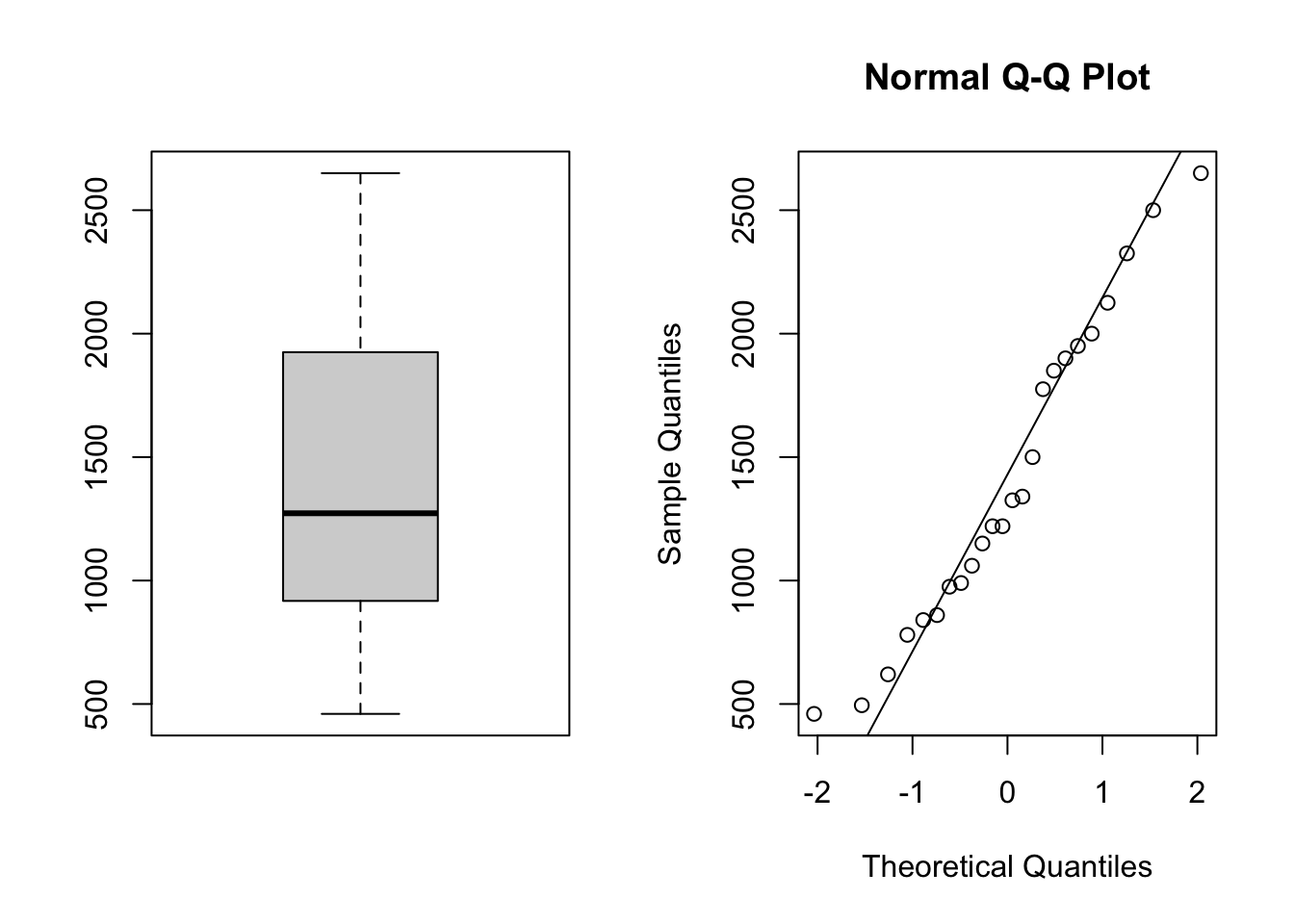
2. Based on the following summary statistics, estimate the standard error for \(\bar{X}\) (assume that the 24 observations are stored in a vector called data)

   c(mean(data), median(data), sd(data), var(data))

   [1]   1412.9167   1272.5000    636.4592 405080.2536

Solution

\[ \sigma_{\bar X} = \text{StError}(\bar X) = \frac{\sigma}{\sqrt{n}} \]

Since we don’t have \(\sigma\) we will estimate this using:

\[ \hat \sigma_{\bar X} = \frac{s}{\sqrt{n}} = \frac{636.4592}{\sqrt{24}} = 129.9166902 \approx 129.917 \]

3. Construct a 90% confidence interval for \(\mu\).

Solution

Using the \(t\)-table with \(n - 1 = 23\) degrees of freedom we want:

\[\begin{align*} \Pr(t_{23} > t^*) &= 0.05\\ \implies t^* &= 1.714 \end{align*}\]

The 90% confidence interval for \(\mu\) is computed using

\[\begin{align*} \bar x &\pm t^* \sigma_{\bar X}\\ 1412.9167 &\pm 1.714 \times 129.917\\ 1412.9167 &\pm 222.677738\\ (1190.239 &,1635.594 ) \end{align*}\] In words, we are 90% confident that the average sulfate S04 in well water is between 1190.2 and 1635.6 in parts per million.

Proportion

Exercise 2.3 In New York City on October 23rd, 2014, a doctor who had recently been treating Ebola patients in Guinea went to the hospital with a slight fever and was subsequently diagnosed with Ebola. Soon thereafter, an NBC 4 New York/The Wall Street Journal/Marist Poll found that 82% of New Yorkers favored a “mandatory 21-day quarantine for anyone who has come into contact with an Ebola patient.” This poll included responses from 1042 New York adults between October 26th and 28th, 2014.

1. What is the point estimate in this case, and is it reasonable to use a normal distribution to model that point estimate?

Solution

The point estimate, based on a sample size of \(n = 1042\), is \(\hat{p} = 0.82\).

To check whether \(\hat{p}\) can be reasonably modeled using a normal distribution, we check:

• Independence (poll is based on a simple random sample)
  
• Success-failure condition:
  • \(n \hat{p} = 1042 \times 0.82 = 854.44 \geq 10\) (condition met)
  • \(n (1 - \hat{p}) = 1042 \times 0.18 = 187.56 \geq 10\) (condition met)

Since both conditions are met, we can assume the sampling distribution of \(\hat{p}\) follows an approxiamte normal distribution.

2. Estimate the standard error of \(\hat{p}\).

Solution

The standard error is given by:

\[ SE_{\hat{p}} = \sqrt{\frac{\hat{p}(1-\hat{p})}{n}} \]

Substituting values:

\[ SE_{\hat{p}} = \sqrt{\frac{0.82(1 - 0.82)}{1042}} = \sqrt{\frac{0.82 \times 0.18}{1042}} \approx 0.012 \]

3. Construct a 95% confidence interval for \(\hat{p}\).

Solution

Using \(SE = 0.012\), \(\hat{p} = 0.82\), and the critical value \(z^* = 1.96\) for a 95% confidence level:

\[\begin{align*} \text{Confidence Interval} &= \hat{p} \pm z^* \times SE \\ &= 0.82 \pm 1.96 \times 0.012 \\ &= 0.82 \pm 0.02352 &\text{ans option 1}\\ &= (0.797, 0.843)&\text{ans option 2} \end{align*}\]

Either the point estimate plus/minus the margin of error, or the confidence interval are acceptable final answers.

4. Interpret the confidence interval.

Solution

We are 95% confident that the proportion of New York adults in October 2014 who supported a quarantine for anyone who had come into contact with an Ebola patient was between 0.797 and 0.843.

5. If we instead wanted an 85% confidence interval, the interval would get
   1. wider
   2. narrower
   3. stay the same
   4. There is not enough information to say

Solution

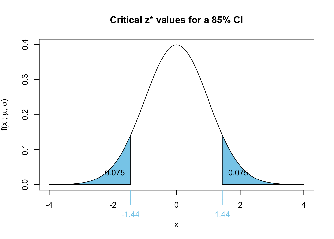
narrower

A lower confidence level corresponds to a smaller \(z^*\) value, which results in a narrower confidence interval.

(a) zstar values

(b) zstar values

Figure 2.2: Left The z* values for a 95% CI. Right The critical z* values of a 85% CI.

Exercise 2.4 A basketball analyst claims that professional players hit free throws at an average rate of 75%. However, some argue that elite players perform better. To investigate, a random sample of 20 elite players was selected. Their individual free throw percentages are given below:

free_throw_perc <- c(84.9, 75.2, 79.8, 81.2, 80, 77.5, 85.6,
                    77.5, 88.1, 77.7, 84.5, 89.4, 71.1, 76.6,
                    77.3, 81.2, 76.6, 64.7, 65.8, 84.6)

Rounding to 1 decmical place to simplify hand calculations, their mean free throw percentage was 79%, with a standard deviation of 6.6%.

Test whether the mean free throw percentage exceeds the league average of 75 percent.

0. Assumptions: Check the assumptions for the appropriate test

Solution

Since there are less than 30 observations, the appropriate test is the one-sample t-test. Recall our flowchart for making this decision:

Since one-sample t-test relies on the following assumptions:

1. Independence of Observations The sample of elite players must be randomly selected, and each player’s free throw percentage should be independent of others. This is primarily determined by study design. If the data was collected randomly and each observation represents a different player, this assumption is likely satisfied.
2. Normality of the Population Distribution: The sample mean follows a t-distribution, but this is valid only if the underlying population is approximately normal or if the sample size is large enough for the Central Limit Theorem (CLT) to apply. There are several ways in which we can check this:
   1. Visual checks:

      1. Histogram (Look for a roughly symmetric, bell-shaped distribution)

         hist(free_throw_perc, breaks = 20)

         

         ⚠️ non-Symmetry: The distribution appears somewhat right-skewed, particularly in the second histogram. We should be weary of this assumption.

      2. Q-Q Plot (Quantile-Quantile Plot): Compare sample quantiles to a theoretical normal distribution.

         I like to use the qqPlot() function from the cars package since it provides some guiding confidence bands which makes it easy to detect deviations.

         # Load necessary library
         library(car)
         # Generate Q-Q plot with confidence bands
         qqPlot(free_throw_perc, main = "Q-Q Plot with Confidence Bands")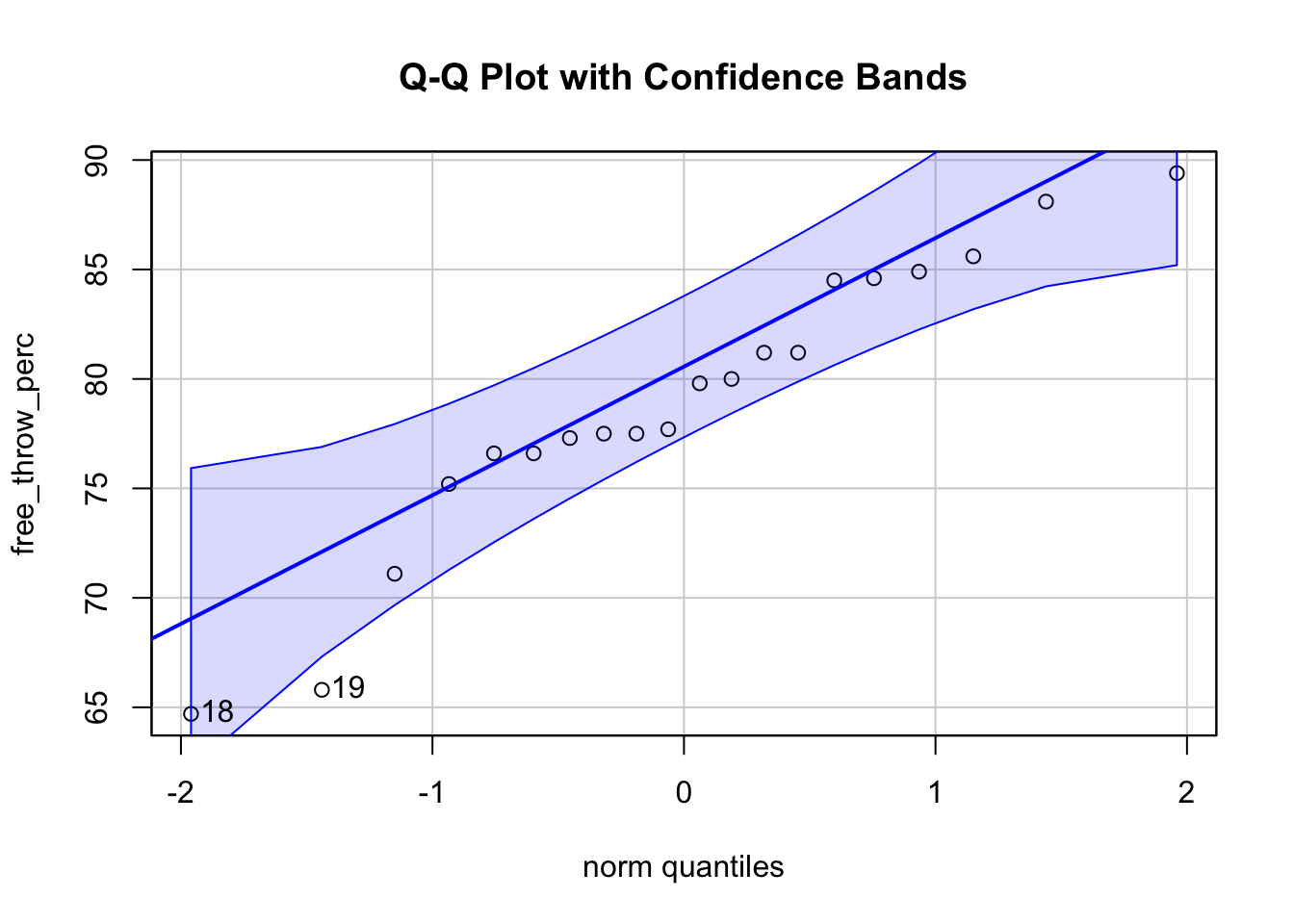

         

         [1] 18 19

         The Q-Q plot with confidence bands shows that most points fall within the bands, indicating approximate normality. There is some deviation in the lower tail (left side) suggests a slight departure from normality, but it isn’t extreme. These correspond to observations (indices) outputted by qqPlot (i.e. observation 18 and 19) are considered potential outliers. That is to say, these are the two most extreme points that deviate from the normality assumption.

      3. Summary:

         • ✅ The Q-Q plot suggests that the data is roughly normal, though there are slight deviations at the lower end.

         • ⚠️ Observations 18 and 19 are flagged as potential outliers, but they are not extreme enough to invalidate the normality assumption.

      4. Shapiro-Wilk Test: A statistical test that checks for normality. If the p-value is greater than 0.05, we do not reject normality.

         shapiro.test(free_throw_perc)

         
             Shapiro-Wilk normality test
         
         data:  free_throw_perc
         W = 0.94389, p-value = 0.2837

         • \(H_0\) : The data follows a normal distribution.

         • \(H_A\) : The data does not follow a normal distribution.

         • p-value: 0.2837 \(> \alpha = 0.05\) \(\implies\) fail to reject

         Conclusion: There is insufficient evidence against normality, and we can reasonably assume that the data is approximately normally distributed.

         Hence we carry on with the one-sample \(t\)-test…

1. Define Hypotheses: State the null and alternative hypothesis:

Solution

We are testing whether the mean free throw percentage of elite players is significantly greater than the league average of 75%.

\[ \begin{align} H_0: &\mu = 75 && H_A: &\mu > 75 \end{align} \]

Hence this is a one-tailed (more specifically a upper-tailed) t-test.

2. Test Statistic: identify the sampling distribution of the test statistic (random variable) and compute the observed test statistic (no longer a random variable).

Solution

Test statistic:

\[ \dfrac{\bar X - \mu_0}{s/\sqrt{n}} \sim t_{\nu = n-1} \]

Hence our test statistic follows a Student-\(t\) distribution with \(\nu = n - 1 = 20 - 1 = 19\) degrees of freedom.

Observed Test Statistic:

\[ \begin{align} t_{obs} &= \dfrac{\bar x - \mu_0}{s/\sqrt{n}}\\ &= \dfrac{79 - 75}{6.6/\sqrt{20}} = 2.71 \end{align} \]

3. Decision:

   1. Decide whether or not the reject \(H_0\) using the critical value method.

      Solution

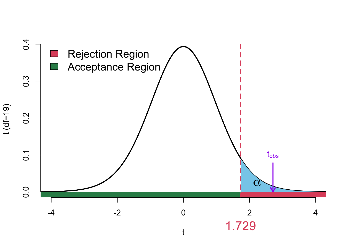
      Critical Value Approach: to use the critical value approach we first need to find the critical values on the null distribution. Hence we need to find \(t^*\) such that

      \[ \Pr(t_{\nu = 19} > t_\alpha^*) = \alpha \] Note that we don’t need to divide \(\alpha\) by two since we are doing the upper-tailed test. The critical value is visualized in Figure 2.3

      

      Figure 2.3: The critical value for an upper-tailed test.

   2. Decide whether or not the reject \(H_0\) using the \(p\)-value approach (this should always agree with the critical value method).

      Solution

      p-value approach

      We need to find

      \[ \Pr(t_{\nu = 19} > 2.71) \]

      Using the \(t\)-tables:

      

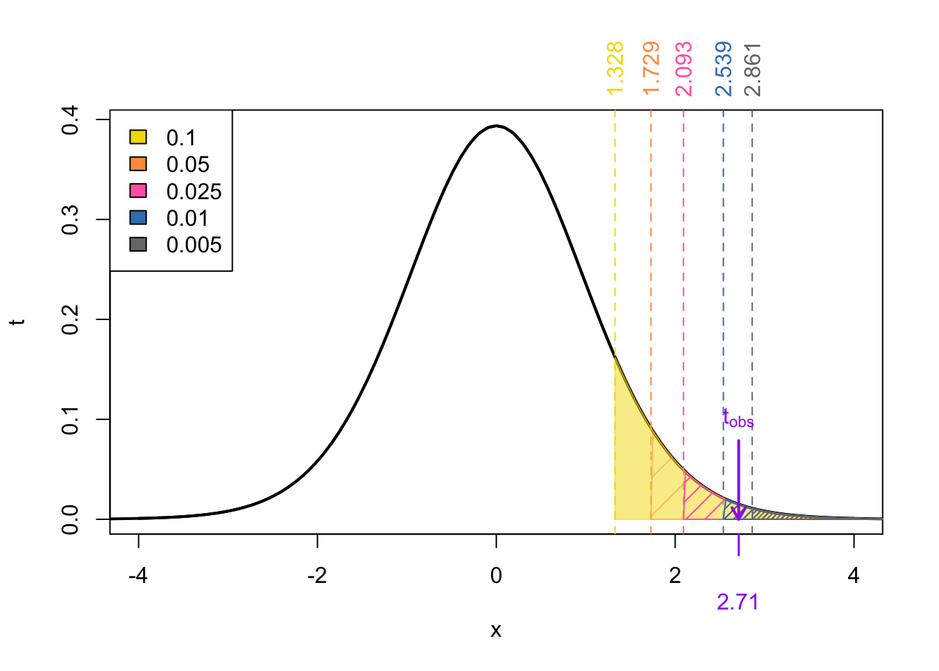
      From the t-tables we can deduce that the \(p\)-value is

      \[ \begin{align} \Pr(t_{\nu = 19} > 2.539) < &\Pr(t_{\nu = 19} > 2.7103854) < \Pr(t_{\nu = 19} > 2.861)\\ \text{area in RoyalBlue }< & p\text{-value} < \text{area in gray}\\ 0.01< & p\text{-value} < 0.005\\ \end{align} \]

      Using R:

      pt(2.7103854, df = 19, lower.tail = FALSE)

      [1] 0.006937378

      Since the \(p\)-value is less than the significance level of \(\alpha\) = 0.05 we reject the null hypothesis.

4. State the appropriate conclusion. Is there evidence that elite players perform better than the league average?

   Solution

   There is strong statistical evidence to suggest that the mean free throw percentage of elite players exceeds the league average of 75%.

Variance

3 Power

Exercise 3.1 Suppose we are about to sample 625 observations from a normally distributed population where it is known that \(\sigma = 100\), but \(\mu\) is unknown. We intend to test:

\[ \begin{align} H_0: \mu &= 500 & H_A: \mu &< 500 \end{align} \] at the \(\alpha = 0.05\) significance level.

(a) What values of the sample mean \(\bar{x}\) would lead to a rejection of the null hypothesis?

Solution

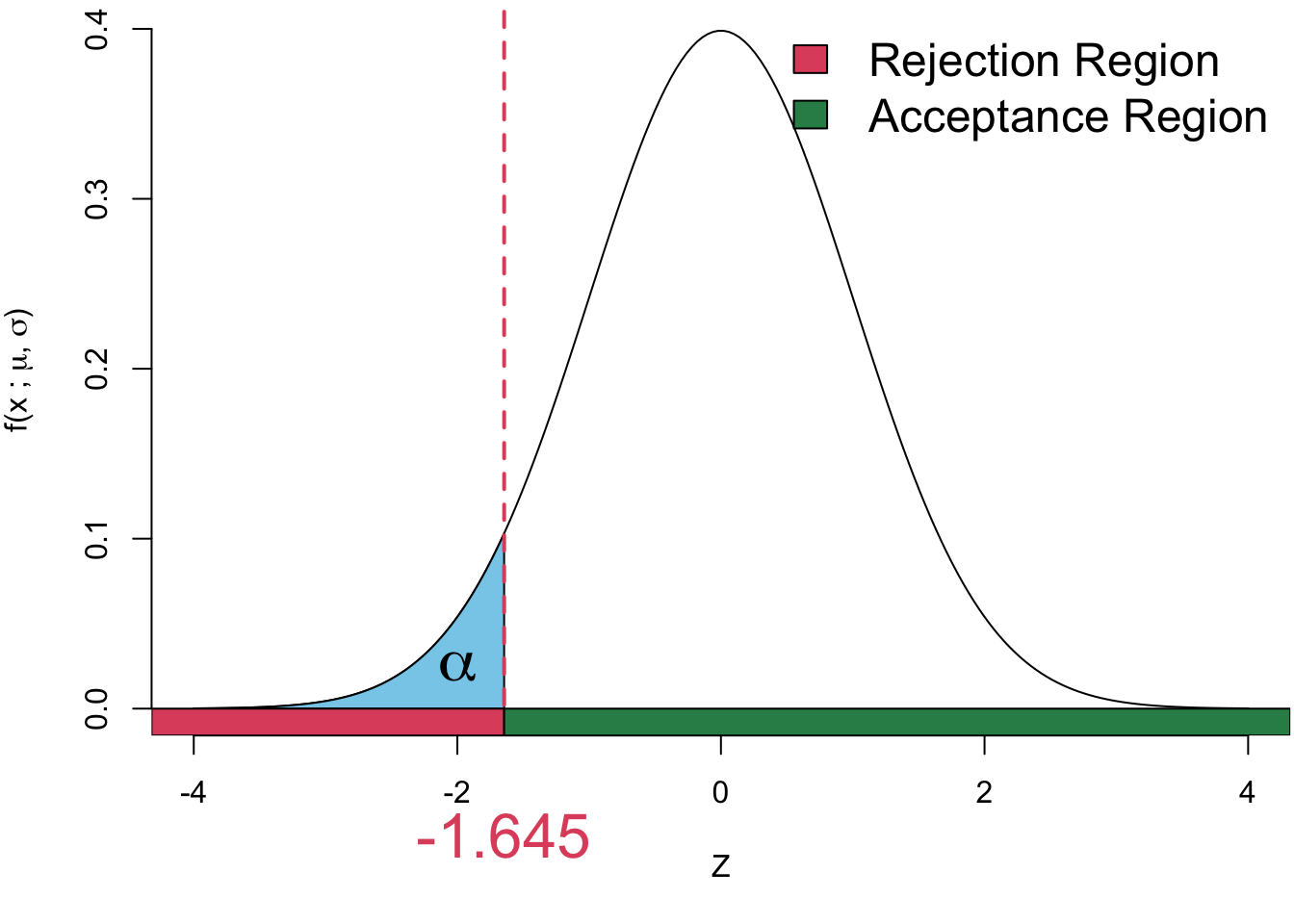
Since this is a left-tailed test, we reject \(H_0\) when the observed test statistic \(\frac{\bar x- \mu_0}{\sigma/\sqrt{n}}\) falls in the rejection region.

Equivalently, we reject the null when \(_\text{obs}\) < the critical value \(z^*\): value:

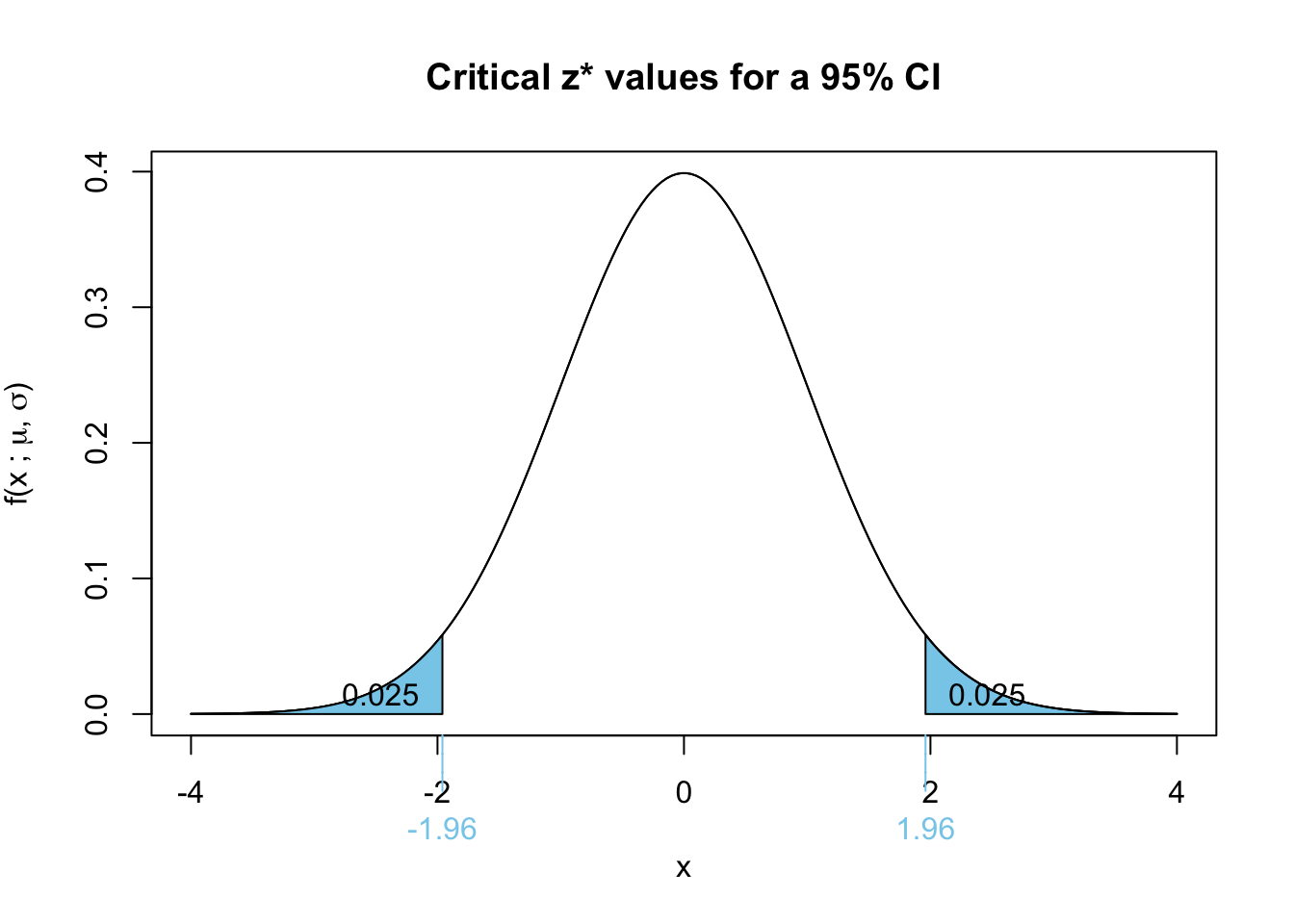
\[ \begin{align} \Pr(Z < z^*) = 0.05\\ \implies z^* = -1.645 \end{align} \]

Convert this to a cutoff for \(\bar{x}\) (which I will denote \(\bar{x}_{crit}\)), we solve:

\[ \begin{align} \text{reject when } z_\text{obs} &< z^*\\ \implies \frac{\bar{x}_{crit} - \mu_0}{\sigma/\sqrt{n}} &= z^*\\ \implies \bar{x}_{crit} &= \mu_0 + z^* \cdot \frac{\sigma}{\sqrt{n}} \\ &= 500 + (-1.645) \cdot \frac{5}{\sqrt{625}}\\ &= 493.42 \end{align} \]

The red region shows values of \(\bar{x}\) that would result in rejection of \(H_0\) at the specified significance level..

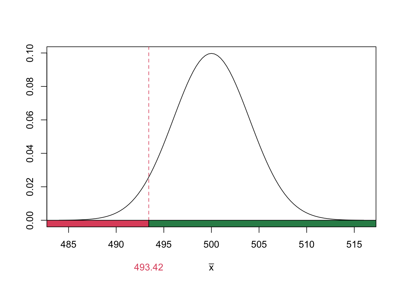
We reject the null hypothesis when \(\bar{x} < 493.42\).

(b) What is the power of the test if the true mean is \(\mu = 490\)?

Solution

We calculate the probability of rejecting \(H_0\) under the alternative \(\mu = 490\). Using the results from (a) and the alternative curve (plotted in orange); I will denot the rv associated with this sampling distribution \(\bar X_A\)

\[ \begin{align} \text{Power} &= \Pr(\text{reject }H_0 \mid H_A \text{ is true})\\ &= \Pr(\bar X_A < \bar x_{\text{crit}}) & \text{where }\textcolor{orange}{\bar X_A \sim N(\mu = 490, \sigma = 4)}\\ &= \Pr\left( \frac{\bar X_A - 490}{\sigma/\sqrt{n}} < \frac{493.42 - 490}{\sigma/\sqrt{n}} \right)\\ &= \Pr(Z < 0.8551464)\\ &= 0.8051 & \text{approximated from the Z-table} \end{align} \]

Finding the power exactly in R we could use:

pnorm(0.8551464)

[1] 0.8037649

Alternative, we could have found the probability without converting to the standard normal by using:

pnorm(493.4205855, mean = 490, sd = 4)

[1] 0.8037649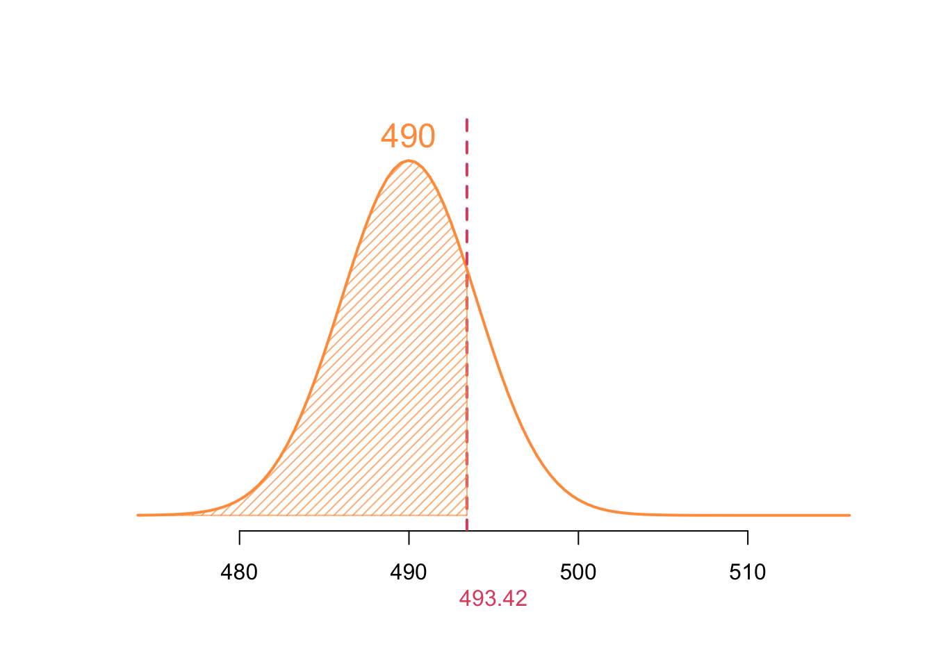

(c) What is the Type II error if the true mean is \(\mu = 490\)?

Solution

This is just the compliment of what we found in part (b); namely:

\[ \begin{align} \Pr(\text{Type II error}) &= \Pr(\text{not rejecting }H_0 \mid H_A \text{ is true})\\ &= 1 - \Pr(\text{rejecting }H_0 \mid H_A \text{ is true})\\ &= 1 - \text{Power}\\ &= 0.1962351 \end{align} \]

The more long winded answer is:

\[ \begin{align} \Pr(\text{Type II error}) &= \Pr(\text{not rejecting }H_0 \mid H_A \text{ is true})\\ &= \Pr(\bar X_A > \bar x_{\text{crit}}) & \text{where }\textcolor{orange}{\bar X_A \sim N(\mu = 490, \sigma = 4)}\\ &= \Pr\left( \frac{\bar X_A - 490}{\sigma/\sqrt{n}} > \frac{493.42 - 490}{\sigma/\sqrt{n}} \right)\\ &= \Pr(Z > 0.8551464)\\ &= 0.1949 & \text{approximated from the Z-table} \end{align} \] Finding the Type II error exactly in R we could use:

pnorm(0.8551464, lower.tail = FALSE)

[1] 0.1962351

Alternative, we could have found the probability without converting to the standard normal by using:

pnorm(493.4205855, mean = 490, sd = 4, lower.tail = FALSE)

[1] 0.1962351

4 Two-Sample Hypothesis Testing

Approximating \(p\)-values using the \(t\)-tables

You will be expected to approximate \(p\)-values using our \(t\)-table. See this document for more details on how to do this.

Mean

Paired

Exercise 4.1 Offerman et al. (2009) conducted an experiment on pigs to investigate the effect of an antivenom after an injection of rattlesnake venom. In one aspect of the study, the researchers investigated the change in volume of the right hind leg before and after being subjected to a dose of venom and treatment with an antivenom. The volume of the right hind leg was measured in 9 pigs before being injected with the venom, then the pigs were injected with a dose of venom and treated intravenously with an antivenom, and after 8 hours the volume of the leg was measured again. The results are illustrated in Table 10.5. (The volume was measured using a water displacement method; the units are mL.)

alpha <- 0.05
diffs <- before - after
n <- length(before)

Exercise 4.2 A fitness coach wants to evaluate the effectiveness of a new treadmill training program on reducing runners’ 5K race times. A sample of r n athletes is timed before and after completing the program:

• Times (in seconds) before: 212, 198, 225, 210, 202, 230, 220, 205, 215, 208

• Times (in seconds) after: 202, 190, 219, 200, 195, 222, 210, 200, 207, 202

At the 5% significance level, is there evidence that the program reduces 5K run times on average?

(a) What type of test is appropriate for this situation?

Solution

A paired t-test is appropriate because the same individuals are measured before and after treatment, making the observations dependent.

(b) State the hypotheses.

Solution

• \(H_0\): The mean difference in run times is zero (\(\mu_d = 0\)).
  
• \(H_A\): The mean difference in run times is greater than zero (\(\mu_d > 0\)), since we’re testing for a reduction in time.

Note: The difference is defined as Before − After, so a positive difference means improvement.

(c) Compute the test statistic by hand.

Solution

We compute the mean and standard deviation of the differences:

before <- c(212, 198, 225, 210, 202, 230, 220, 205, 215, 208)
after  <- c(202, 190, 219, 200, 195, 222, 210, 200, 207, 202)
diffs <- before - after

n <- length(before)
xbar <- mean(diffs)
s <- sd(diffs)
se <- s / sqrt(n)
tstat <- xbar / se
nu <- n - 1
pval <- pt(tstat, nu, lower.tail = FALSE)
reject = pval < alpha

• \(\bar{d} = 7.8\)
  
• \(s_d = 1.814\)
  
• \(n = 10\)
  
• \(\text{SE} = \frac{s_d}{\sqrt{n}} = \frac{1.814}{\sqrt{10}} = 0.573\)

Test statistic:

\[ t = \frac{\bar{d} - 0}{\text{SE}} = \frac{7.8}{0.573} = 13.601 \]

(d) Calculate the p-value i) approximate using the \(t\)-tables ii) exactly using R.

Solution

We need to refer to the \(t\)-table with \(\nu = n-1 = 10 -1 = 9\). There reference row is depicted below:

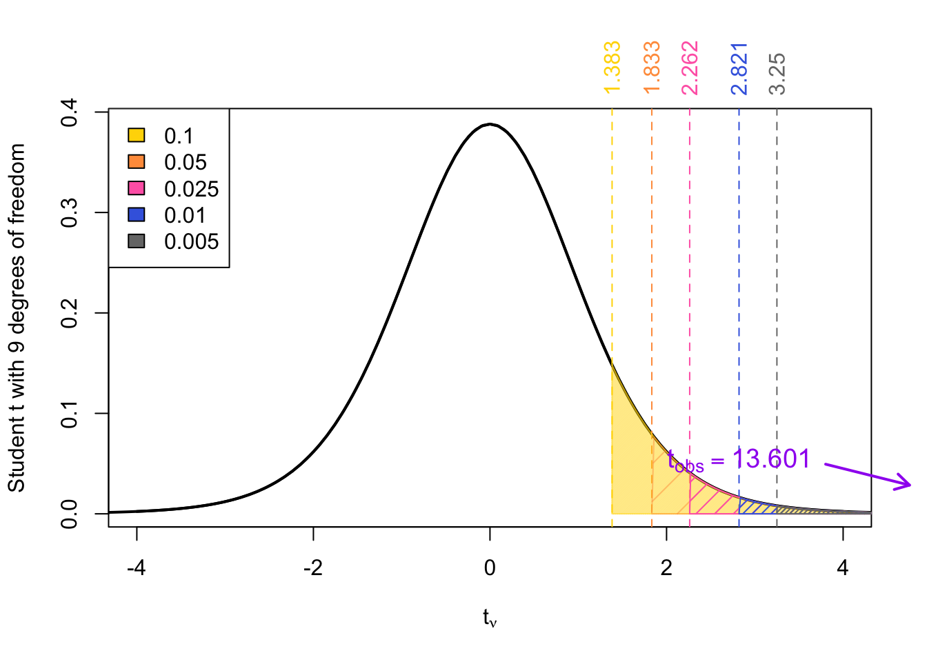
With an observed test statistic of 13.601, the \(p\)-value is approximated as:

\[ \begin{align} p\text{-value} &= \Pr(t_{9} > t_\text{obs} ) \\ &= \Pr(t_{9} > 13.6) \\ & < \Pr(t_{9} > \textcolor{gray}{3.25}) = \textcolor{gray}{0.005} \\ \implies p\text{-value} &< \textcolor{gray}{0.005} \end{align} \]

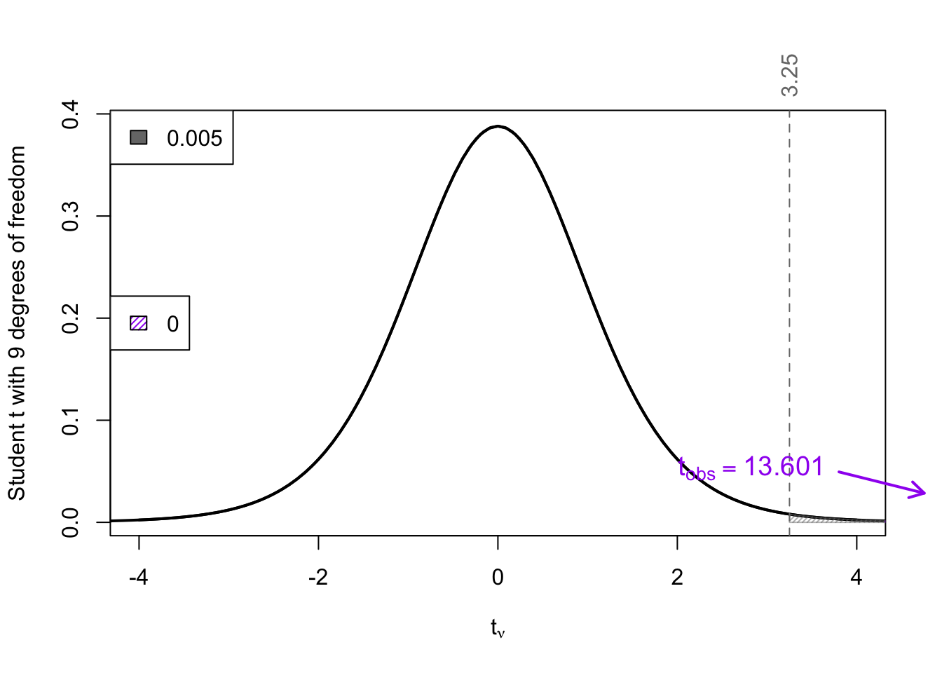
The null distribution is a Student \(t\) with degrees of freedom: \(df = n - 1 = 9\). The exact \(p\)-value is calculated using:

pt(13.601, df = 9, lower.tail = FALSE)

[1] 1.316055e-07

The relationship between the exact \(p\)-value and the relant reference \(t\)-values is shown below. As we can see,

\[ p\text{-value} = 0.0000001316055 < \textcolor{gray}{0.005} \]

(e) State your decision.

Solution

Since the p-value is less than \(\alpha = 0.05\), we reject the null hypothesis.

There is sufficient evidence to conclude the treadmill program reduces average 5K run times.

Pooled

Exercise 4.3 A researcher wants to compare the average weight (in pounds) of two breeds of small dogs. A random sample of dogs from each breed is selected:

• Breed A: 160, 165, 158, 170, 162, 164, 159

• Breed B: 155, 150, 158, 152, 149, 153, 151

Assume the population variances for the two breeds are equal. At the 5% significance level, is there evidence that the mean weights of the two breeds differ?

(a) What kind of test is appropriate?

Solution

A two-sample pooled \(t\)-test is appropriate because we are comparing the means of two independent samples and we assume equal population variances.

(b) State the hypotheses.

Solution

Let \(\mu_1\) and \(\mu_2\) represent the population mean weights for Breed A and Breed B respectively.

\[\begin{align} H_0: & \ \mu_1 = \mu_2 & H_A: & \ \mu_1 \ne \mu_2 \end{align}\]

This is a two-sided test.

(c) Compute the test statistic by hand.

Solution

We first compute the pooled standard deviation:

\[ s_p = \sqrt{ \frac{(n_1 - 1)s_1^2 + (n_2 - 1)s_2^2}{n_1 + n_2 - 2} } = \sqrt{ \frac{(6) \cdot 17.29 + (6) \cdot 9.62}{12} } = 3.668 \]

Then the standard error:

\[ SE = s_p \cdot \sqrt{\frac{1}{n_1} + \frac{1}{n_2}} = 3.668 \cdot \sqrt{\frac{1}{7} + \frac{1}{7}} = 1.96 \]

Finally, the test statistic:

\[ t_{obs} = \frac{\bar{x}_1 - \bar{x}_2}{SE} = \frac{162.57 - 152.57}{1.96} = 5.101 \]

(d) State the null distribution.

Solution

Under \(H_0\), the test statistic follows a \(t\) distribution with \(\nu = n_1 + n_2 - 2 = r nu\) degrees of freedom.

(e) Use the critical value approach to make a decision.

Solution

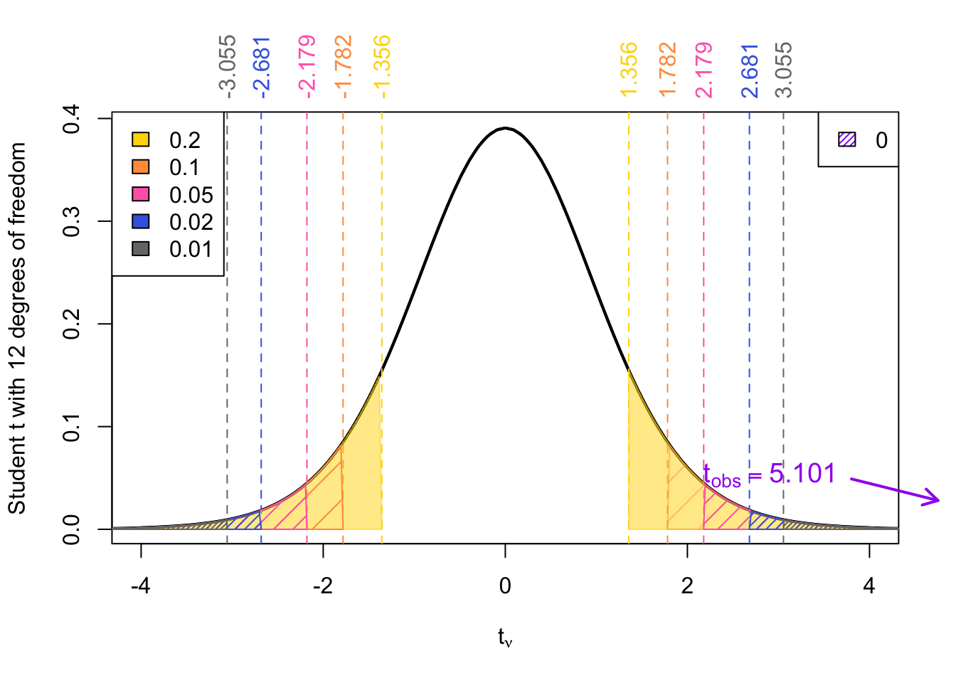
For a two-sided test at \(\alpha = 0.05\), the critical value is:

\[ t^* = t_{\alpha/2, \nu} = t_{0.025, 12} = 2.179 \]

We reject the null hypothesis if \(|t_{obs}| > t^*\):

\[ |5.101| > 2.179 \]

So we reject the null hypothesis.

Visually we can see that our observed test statistic falls in the rejection region. Hence we reject the null in favour of the alternative.

rr_t(df = nu, symbols = FALSE)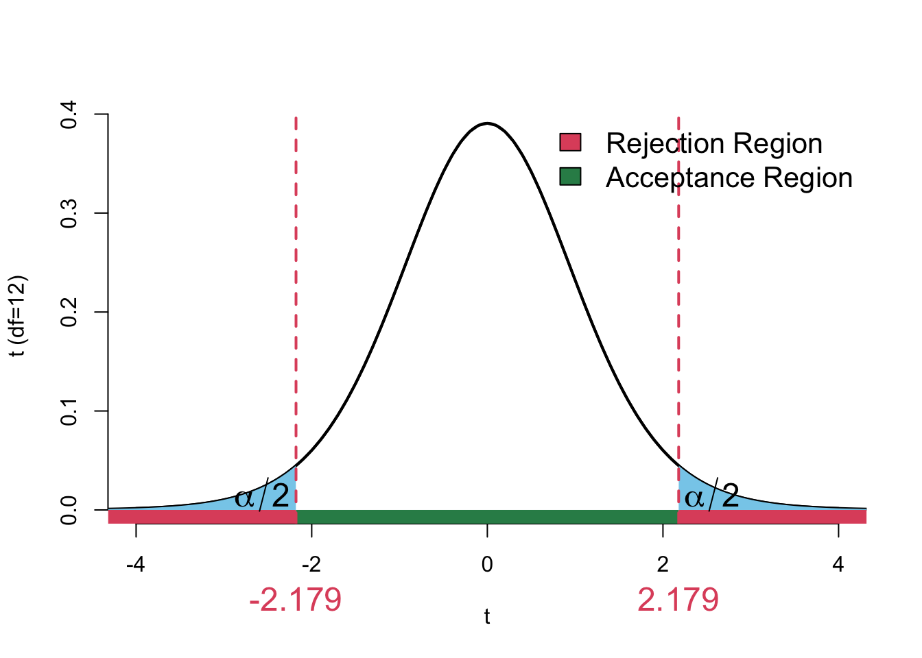

(f) Compute the p-value i) approximate using the t-tables ii) exactly using R.

Solution

The reference row from the \(t\)-table is:

Given a \(t_{obs}\) = 5.1007548 degrees of freedom \(\nu\) = 12 the \(p\)-value can be approximated as:

\[ \begin{align} p\text{-value} &= 2 \times \Pr(t_{12} > t_\text{obs} ) \\ &= 2 \times \Pr(t_{9} > 5.1) \\ & < 2 \times \Pr(t_{9} > \textcolor{gray}{3.25}) = 2 \times \textcolor{gray}{0.005} \\ \implies p\text{-value} &< \textcolor{gray}{0.01} \end{align} \]

The exact \(p\)-value is found using:

2*pt(abs(5.1007548), df = 12, lower.tail = FALSE)

[1] 0.0002614753

Hence: \[ p = 2 \cdot \Pr(t_{\nu = 12} > |t_{obs}|) = 2 \cdot \Pr(t_{12} > 5.101) = 2.61e-04 \]

Visually:

Welch

Proportions

5 ANOVA

Exercise 5.1 Researchers are investigating the effect of different treatments on plant growth. The dataset PlantGrowth contains the weights of plants subjected to three different groups: a control group (ctrl), and two treatment groups (trt1 and trt2). Each group contains 10 observations (30 total). A box plot of the data is provided in Figure 5.1.

PlantGrowth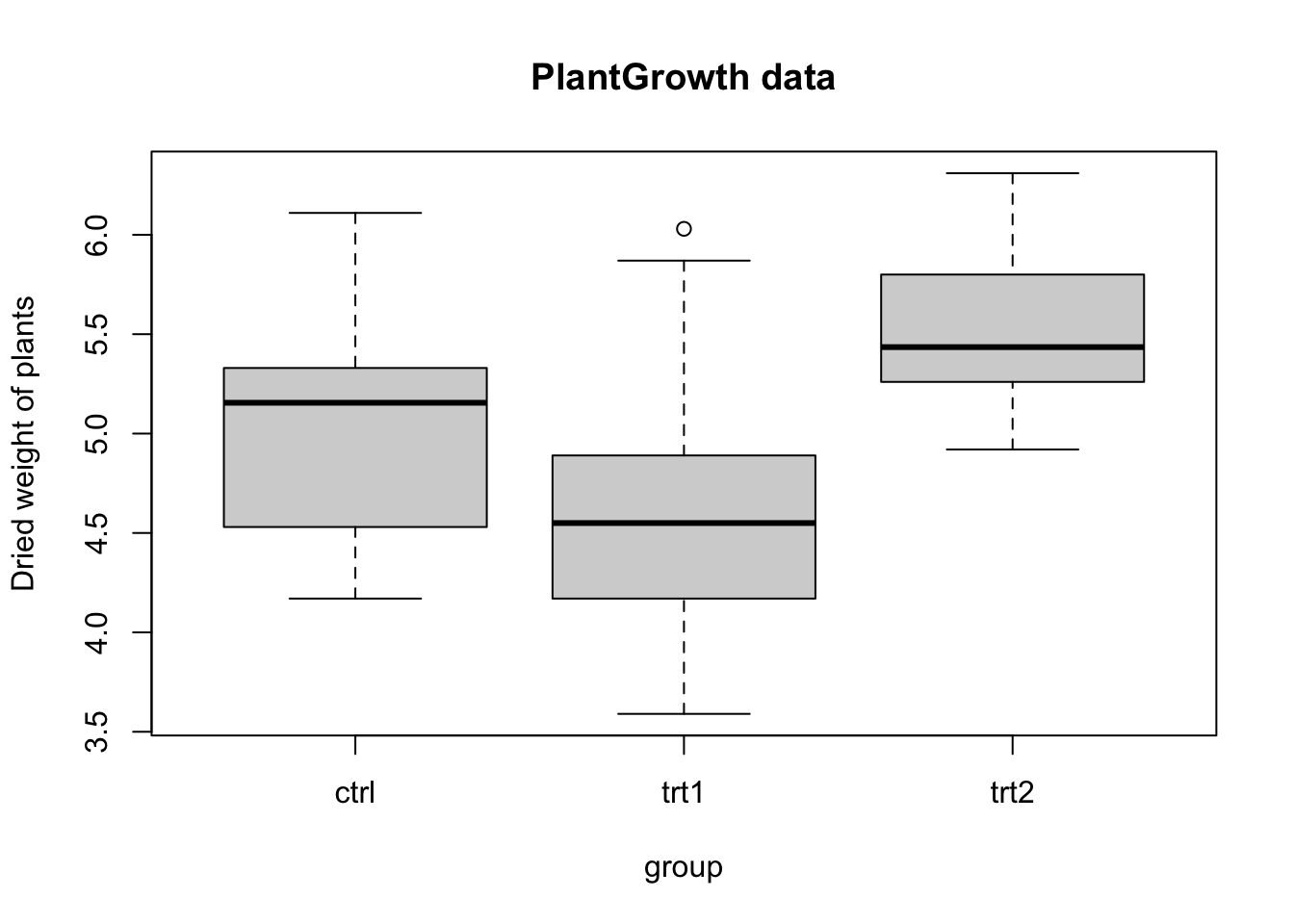

Figure 5.1

A one-way ANOVA was performed in R using the code below:

anova_result <- aov(weight ~ group, data = PlantGrowth)
summary(anova_result)

Source	Df	Sum Sq	Mean Sq	F value	Pr(>F)
group		3.7663			0.0159
Residuals			0.3886

(a) Complete the ANOVA table (you have enough information to complete the table without having to refer to the dataset help file or R for examining the output).

Solution

To complete the ANOVA table, we use the following information and formulas:

• Total number of observations: \(n = 30\)
• Degrees of freedom:
  • \(\text{df}_{\text{group}} = 3 - 1 = 2\)
  • \(\text{df}_{\text{residual}} = 30 - 3 = 29\)

We are given:

• \(\text{SS}_{\text{group}} = 3.7663\)
• \(\text{MS}_{\text{residual}} = 0.3886\)
• \(\text{p-value} = 0.0159\)

NOTE: If the \(p\)-value was missing, we it could be found using

pf(4.8461, df1 = 2, df2 = 27, lower.tail = FALSE)

[1] 0.01590982

We now compute:

Mean Square for group

\[ \text{MS}_{\text{group}} = \frac{\text{SS}_{\text{group}}}{\text{df}_{\text{group}}} = \frac{3.7663}{2} = 1.8832 \]

Sum of Squares for residuals:

\[ \text{SS}_{\text{residual}} = \text{MS}_{\text{residual}} \times \text{df}_{\text{residual}} = 0.3886 \times 27 = 10.4921 \]

F statistic:

\[ F = \frac{\text{MS}_{\text{group}}}{\text{MS}_{\text{residual}}} = \frac{1.8832}{0.3886} = 4.8461 \]

Source	Df	Sum Sq	Mean Sq	F value	Pr(>F)
group	2	3.7663	1.8832	4.8461	0.0159
Residuals	27	10.4921	0.3886

(b) What is the null and alternative hypothesis being tested by this ANOVA?

Solution

The null hypothesis is that the mean plant weights are equal across all three groups. Formally: \[ H_0: \mu_\text{ctrl} = \mu_\text{trt1} = \mu_\text{trt2} \quad \quad \] That is, there is no difference in mean plant weight between the control group and the two treatment groups.

vs. the alternative:

\[ H_A: \text{At least one } \mu_i \text{ is different} \] In other words, the alternative states At least one treatment group has a significantly different mean plant weight.

(c) At the \(\alpha = 0.05\) significance level, what conclusion should be drawn based on the ANOVA result? Interpret it in context.

Solution

The p-value from the ANOVA is 0.0159, which is less than \(\alpha = 0.05\). Therefore, we reject the null hypothesis.

This suggests that at least one of the treatment groups has a significantly different mean plant weight compared to the others.

(d) What follow-up analysis should the instructor conduct to determine which specific groups differ in exam performance? Explain its purpose.

Solution

While we have discovered that there is significant difference between at least one of the group means, we do not know which group is significantly differnt. While we can probably guess from the boxplot, we can conduct some post-hoc analysis that compares all possible pairs of group means and adjusts for multiple comparisons. Its purpose is to determine which specific pairs of groups (e.g., ctrl vs. trt1, trt1 vs. trt2, or ctrl vs. trt2) differ significantly in mean plant weight.

(e) ANOVA relies on several assumptions. Name one assumption and describe how it could be verified.

Solution

Assumption: Homogeneity of variances — the population variances are equal across groups.

This can be checked using:

• A residuals vs. fitted plot — to assess if the spread of residuals is roughly constant across all fitted values.
• Boxplots of plant weight by group — to visually compare the variability (spread) in each group.
• Levene’s test or Bartlett’s test (not graphical but formal tests for equal variance).

another option could be:

Assumption: Independence of Observations – Each data point is unrelated to the others (e.g., no pairing or repeated measures).

How to check:

• Not directly checkable via plots.
• Must be ensured through study design (e.g., proper randomization and independent sampling).

6 Chi-squared tests

Test for Independence

Exercise 6.1 Suppose we want to test the effectiveness of a drug for a certain medical condition. We have 105 patients under study and 50 of them were treated with the drug, and the remaining 55 patients were kept under control samples. The health condition of all patients was checked after a week.

data_frame = read.csv("https://goo.gl/j6lRXD")
table(data_frame$treatment, data_frame$improvement)

             
              improved not-improved
  not-treated       26           29
  treated           35           15

In the contingency table we see that 35 out of the 50 patients in the treatment group showed improvement, compared to 26 out of the 55 in the control group. Perform the appropriate chi-squared test for independence

1. by hand

2. using R’s chi.test() function

Solution

• If the drug had no effect, we would expect the same proportion of the patients who improved to be the same between the treatment and control group.

• Here, the improvement in the treatment case is 70% , as compared to 47.27 % in the control group.

• Do these data ssuggest that the drug treatment and health condition are dependent?

• A chi-squared test for independence will examine the relationship between two categorical variables: treatment condition (drug vs. control) and health outcome (improvement vs. no improvement).

Hypotheses

• \(H_0\): Health outcome of patients is independent of whether or not the patient took the drug
• \(H_A\): Health outcome of patients depends on whether or not the patient took the drug

Other ways you might say this:

• \(H_0\): There is no association between the treatment condition and the health outcome of the patients.
• \(H_A\): There is an association between the treatment condition and the health outcome of the patients.

The null implies that the drug does not affect the health outcome of the patients compared to the control group.

The alternative implies that the drug has an effect on the health outcome, making an improvement more likely (or less likely) compared to the control group.

To answer this question we need to compute the expected table. Under the null, the expected counts would be:

\[ \dfrac{\text{row total} \times \text{col total}}{\text{total}} \]Below I have computed the corresponding sums and added them to the margins:

             response
treatment     improved not-improved Sum
  not-treated       26           29  55
  treated           35           15  50
  Sum               61           44 105

The calculations performed cell by cell are as follows:

\[ \begin{align} \text{Expected no. of not-treated that improved } &= \dfrac{55 \times 61}{105} = 31.952381\\ \text{Expected no. of not-treated that not-improved } &= \dfrac{55 \times 44}{105} = 23.047619\\ \text{Expected no. of treated that improved } &= \dfrac{50 \times 61}{105} = 29.047619\\ \text{Expected no. of treated that not-improved } &= \dfrac{50 \times 44}{105} = 20.952381 \end{align} \]

             response
treatment     improved not-improved
  not-treated 31.95238     23.04762
  treated     29.04762     20.95238

To calculate the test statistic we compute our test statistic

\[ \sum \dfrac{(\text{Observed} - \text{Expected})^2}{\text{Expected}} \sim \chi^2_{df = 2 \times \nu_2 = 1 = 1} \]

\[ \begin{align} \\ &= \frac{(26 - 31.952381)^2}{31.952381} + \frac{(29 - 23.047619)^2}{23.047619} + \dots\\ &\quad \dots \frac{(35 - 31.952381)^2}{29.047619} + \frac{(15 - 31.952381)^2}{20.952381}\\ &= 5.5569198 \end{align} \]

Comparing this to a \(\chi^2\) random variable with \(df = (r - 1) \times (c -1)\) \((2 - 1) \times (2 - 1) = 1\)

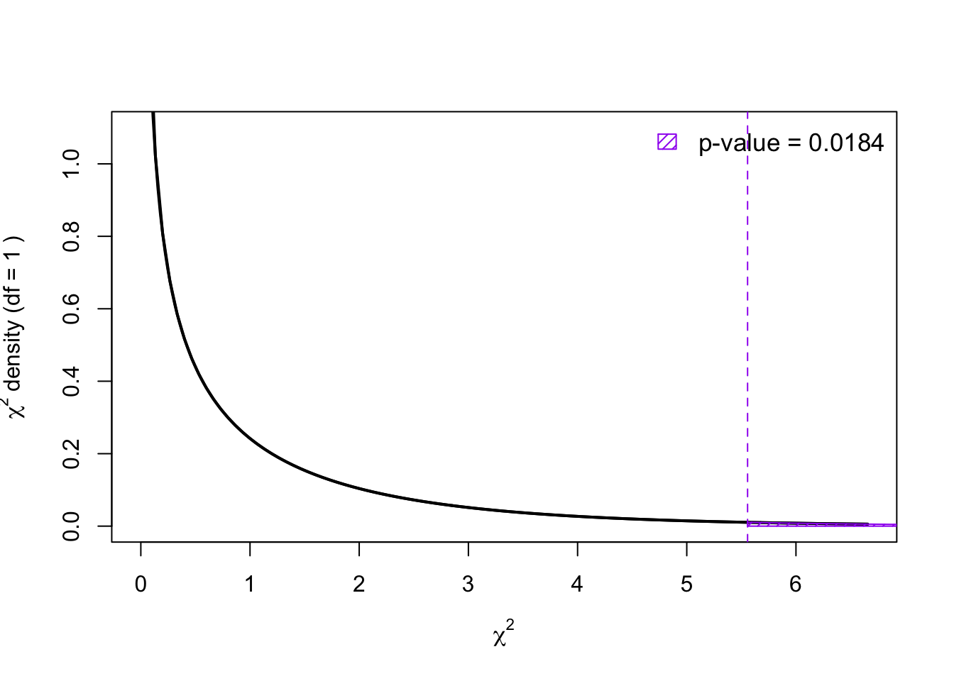
Since the \(p\)-value is less than the significance level of \(\alpha = 0.05\), we reject the null hypothesis in favour of the alternative. Hence there is sufficient statistical evidence to suggest that Health outcome of patients is indepedent of whether or not the patient took the drug.

2. do this again using the R chisq.test() function

In the case of a null hypothesis, a chi-square test is to test the two variables that are independent. The following conducts a a chi-squared test on the treatment and improvement

chisq.test(data_frame$treatment, data_frame$improvement, correct=FALSE)

To match the results above we use correct=FALSE to turn off the continuity correction (where one half is subracted from all observed - expected differences).

Goodness of Fit

Exercise 6.2 car manufacturer claims that the proportion of defective brake pads produced across its three work shifts is consistent with historical rates: 20% during the day shift, 30% during the evening shift, and 50% during the night shift.

To assess this claim, a quality control manager inspects a random sample of 200 defective brake pads and records which shift they came from:

• Day shift: 30
• Evening shift: 50
• Night shift: 120

At the 5% significance level, is there evidence that the current distribution of defects differs from the historical pattern?

1. What are the null and alternative hypotheses?

Solution

• \(H_0\): The distribution of defects follows the historical proportions: \(p = (0.2, 0.3, 0.5)\)
  
• \(H_A\): The distribution of defects does not follow the historical proportions.

2. What is the null distribution associated with this test

Solution

The chi-squared test statistic is

\(\chi^2 = \sum \frac{(O_i - E_i)^2}{E_i}\)

which follows a Chi-squared distribution with \(\nu\) =3- 1 =2 degrees of freedom.

3. Compute the chi-squared test statistic.

Solution

Under the null hypothesis, the expected counts are:

• Day: \(E_1 = 200 \times 0.2 = 40\)
  
• Evening: \(E_2 = 200 \times 0.3 = 60\)
  
• Night: \(E_3 = 200 \times 0.5 = 100\)

The chi-squared test statistic is calculated using the formula:

\(\chi^2 = \sum \frac{(O_i - E_i)^2}{E_i}\)

Substituting the observed and expected values:

\(\chi_{obs}^2 = \frac{(30 - 40)^2}{40} + \frac{(50 - 60)^2}{60} + \frac{(120 - 100)^2}{100} = 8.167\)

4. Make a decision based on the critical value method

Solution

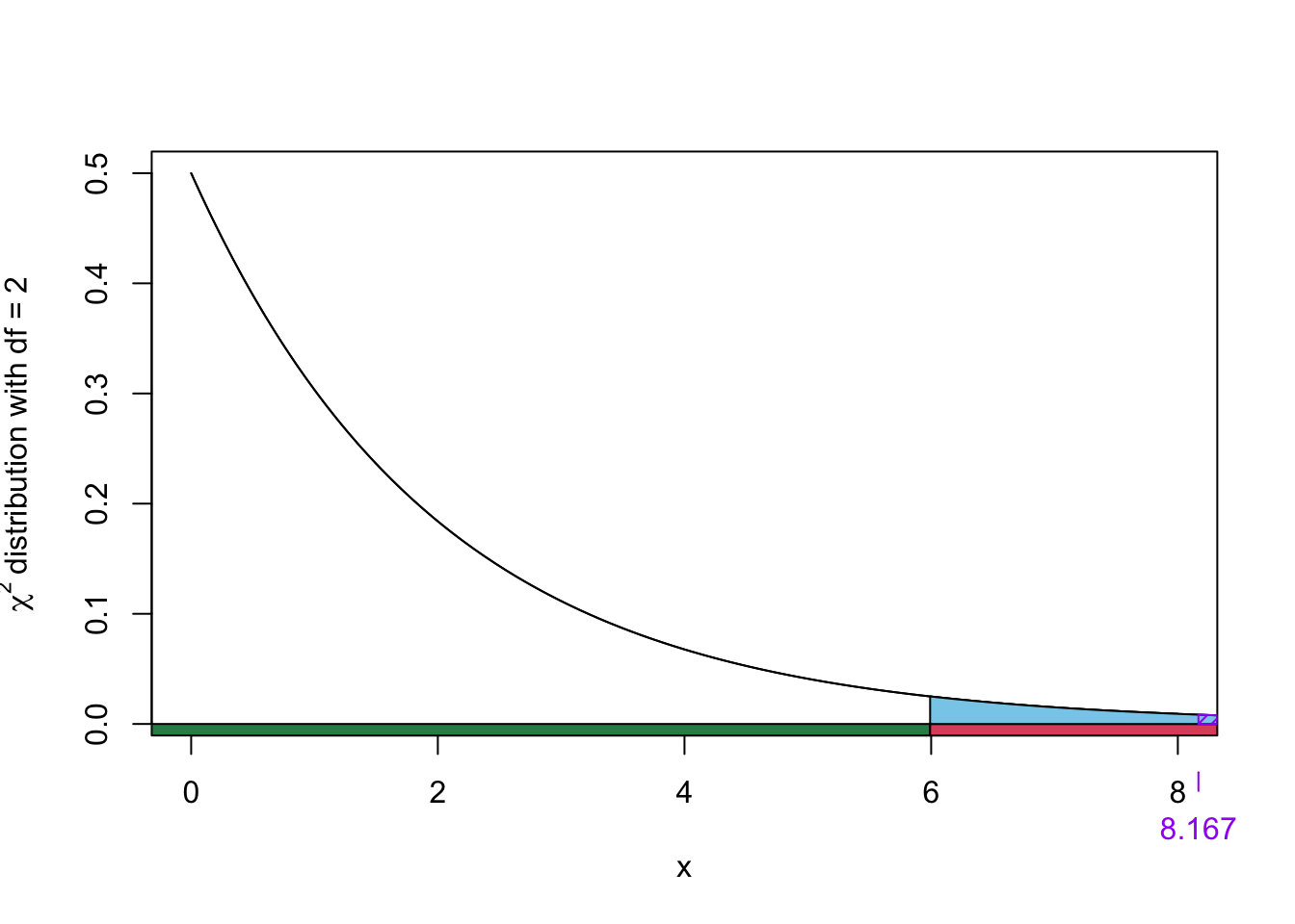
Since the observed test statistic \(\chi^2_{obs}\) = 8.1666667 falls inside the rejection rejection, we reject the null hypothesis in favour of the alternative.

5. Compute the \(p\)-value i) approximately using the tables ii) exactly using R.

Solution

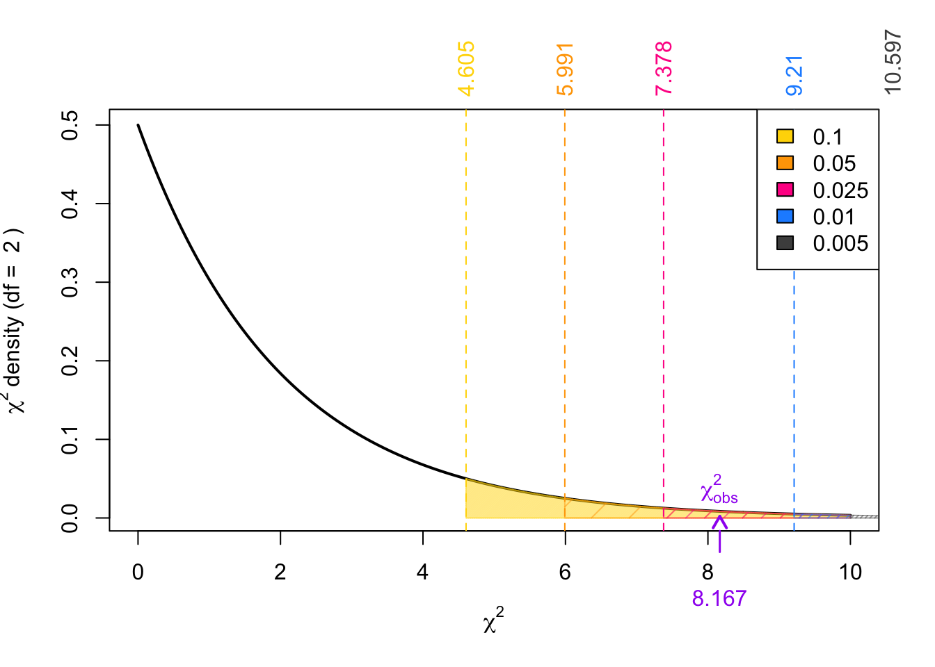
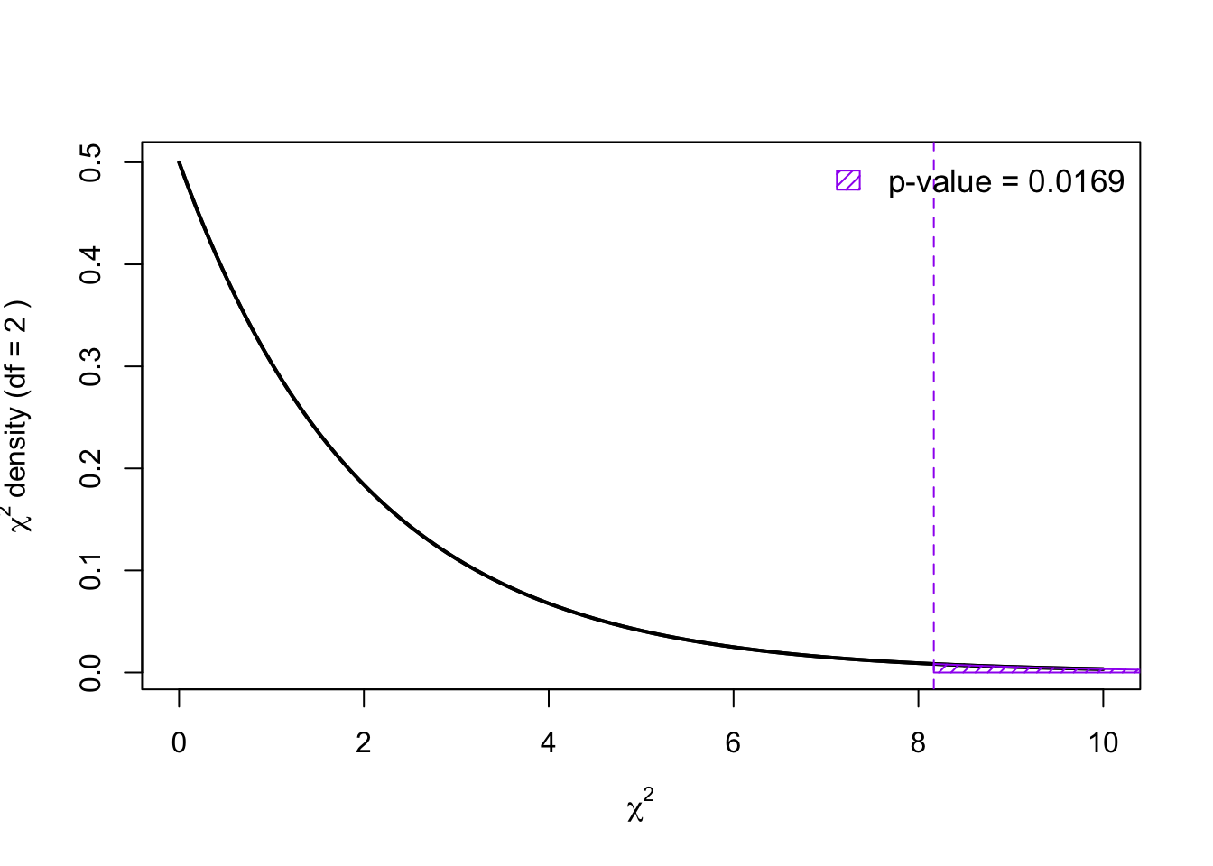
The exact p-value in R is computed using

pchisq(8.1666667, df = 2, lower.tail = FALSE)

[1] 0.0168512

6. Sketch the \(p\)-value

Solution

Remember that the chi-squared tests are always upper-tailed test. The p-value is visualized below:

7. State the conclusion for this test

Solution

Since the \(p\)-value is less than \(\alpha = 0.05\), we reject the null hypothesis.

There is sufficient evidence to conclude that the current distribution of defective brake pads differs from the historical pattern.

h. Which of the following R commands correctly performs a chi-squared goodness-of-fit test for this scenario?

1. chisq.test(30, 50, 120)
2. chisq.test(30, 50, 120, p = c(1/3, 1/3, 1/3))
3. chisq.test(30, 50, 120, p =0.2, 0.3, 0.5)
4. chisq.test(0.2, 0.3, 0.5, p =30, 50, 120)

Solution

By default, chisq.test() assumes a uniform distribution — meaning it tests whether all categories occur equally often. So if you just run:

chisq.test(30, 50, 120)

it tests whether all three shifts produce an equal number of defects (i.e., 1/3 each).

But in this case, the company has provided specific expected proportions:

• 20% during the day
• 30% during the evening
• 50% during the night

To incorporate those values, we use the p argument in chisq.test():

chisq.test(30, 50, 120, p =0.2, 0.3, 0.5)

    Chi-squared test for given probabilities

data:  observed
X-squared = 8.1667, df = 2, p-value = 0.01685

This tells R to compare the observed counts to the non-uniform expected distribution. So iii. is correct

Test for Homogenity

Exercise 6.3 An automobile manufacturer wants to know whether three factories produce the same distribution of defect types.

A random sample of recent defects at each factory is recorded below:

          Brake Steering Transmission
Factory A    35       15           25
Factory B    22       18           20
Factory C    28       12           30

At the 5% significance level, is there evidence that the distribution of defect types differs across the three factories?

(a) State the hypotheses.

Solution

• \(H_0\): The distribution of defect types is the same across all three factories.
  
• \(H_A\): The distribution of defect types is not the same across all three factories.

(b) What type of test is appropriate for this situation? i. Chi-squared test for independence ii. Chi-squared goodness of fit test iii. Chi-squared test for homogenity iv. None of the above are appropriate

Solution

A Chi-squared test for homogeneity is appropriate because we are comparing the distribution of a categorical variable (defect type) across different populations (factories).

(c) Conduct the appropriate test in R.

Solution

Use:

chisq.test(counts)

    Pearson's Chi-squared test

data:  counts
X-squared = 4.6398, df = 4, p-value = 0.3263

This will output the test statistic, degrees of freedom, and p-value. R treats the rows as different groups (factories) and tests whether the column proportions (defect types) are the same across groups.

(d) State your conclusion based on the \(p\)-value and \(\alpha = 0.05\).

Solution

Since the \(p\)-value is greater than \(\alpha = 0.05\), we fail to reject the null hypothesis . Hence, there is insufficient statistical evidence to conclude that the distribution of defect types differs across factories.