Approximate \(p\)-values using \(t\)-tables

STAT 205: Introduction to Mathematical Statistics

Author

Affiliation

Dr. Irene Vrbik

University of British Columbia Okanagan

The document explains how we can approximate \(p\)-values from the \(t\)-table.

Steps for Computing \(p\)-values from \(t\)-tables

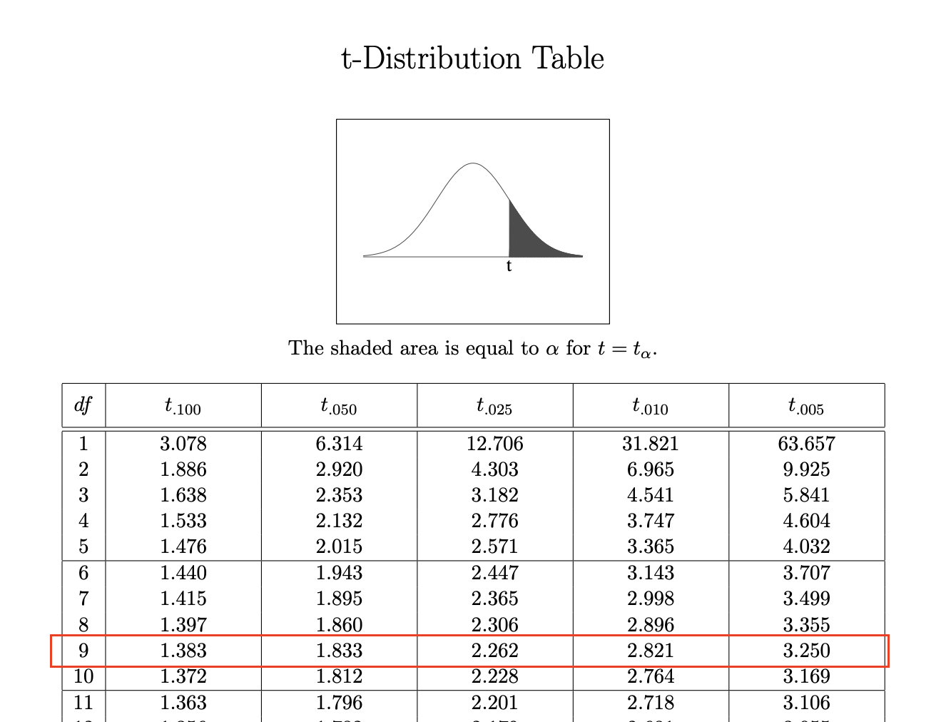
Step 1: Locate your degrees of freedom

Find the row in the table that matches your degrees of freedom (\(\nu\)).

Conservative degrees of freedom

If your \(\nu\) is not listed, use the next lowest available value to be conservative. - Example: If \(\nu = 33\) and the table includes 32 and 34, use \(\nu = 32\).

Step 2: Find the reference \(t\)-values

On the row for your chosen \(\nu\), you’ll find five reference values corresponding to common upper-tail probabilities:

\[ t_{0.1}, t_{0.05}, t_{0.025}, t_{0.01}, t_{0.005} \]

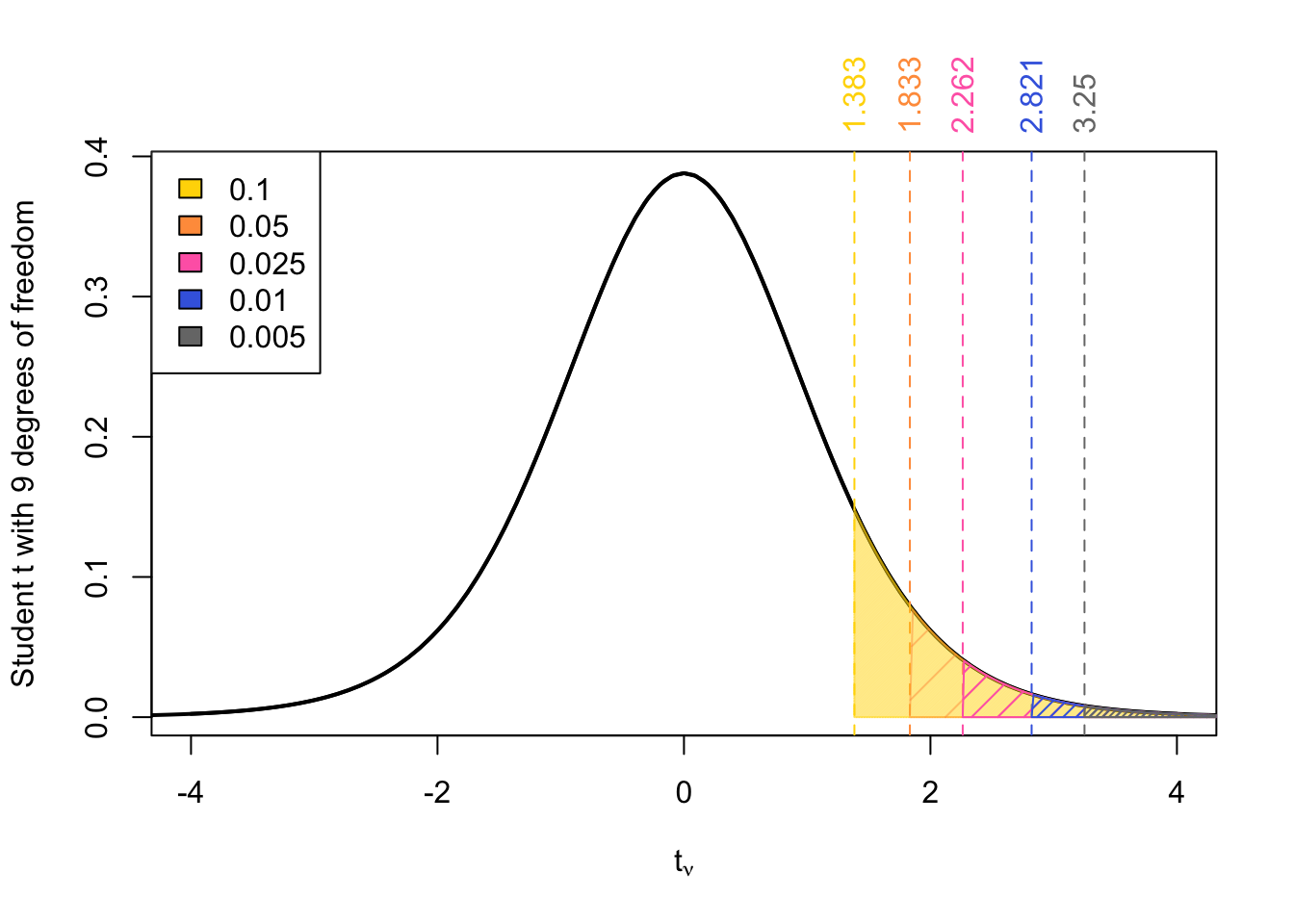
For example, if we examine the row of the \(t\)-table with 9 degrees of freedom, we get the reference values: \(t_{0.1} = 1.383, t_{0.05}= 1.833, t_{0.025} = 2.262, t_{0.01} = 2.821, t_{0.005} = 3.25\)

Step 3: Compare your test statistic \(t_\text{obs}\) to the reference values

For upper-tailed \(p\)-values

• If \(t_{\text{obs}}\) falls between two reference values in the row → the \(p\)-value falls between the corresponding probabilities shown at the top of the columns.
• If \(t_{\text{obs}}\) is greater than all reference values in the row → the \(p\)-value is less than the smallest probability listed (0.005).
• If \(t_{\text{obs}}\) is smaller than all values → the \(p\)-value is greater than the largest probability listed.

This plot shows the upper-tail probabilities of a \(t\)-distribution with 9 degrees of freedom. Vertical dashed lines mark the reference \(t\)-values corresponding to common probabilities in the upper-tail (\(0.1\), \(0.05\), \(0.025\), \(0.01\), and \(0.005\)) as indicated by the shaded regions.

For lower-tailed \(p\)-values

For lower-tailed tests, simply apply the same logic using the negative of the reference \(t\)-values for the appropriate degrees of freedom.

This plot shows the lower-tail probabilities of a \(t\)-distribution with 9 degrees of freedom. Vertical dashed lines mark the reference \(t\)-values corresponding to common probabilities in the upper-tail (\(0.1\), \(0.05\), \(0.025\), \(0.01\), and \(0.005\)) as indicated by the shaded regions.

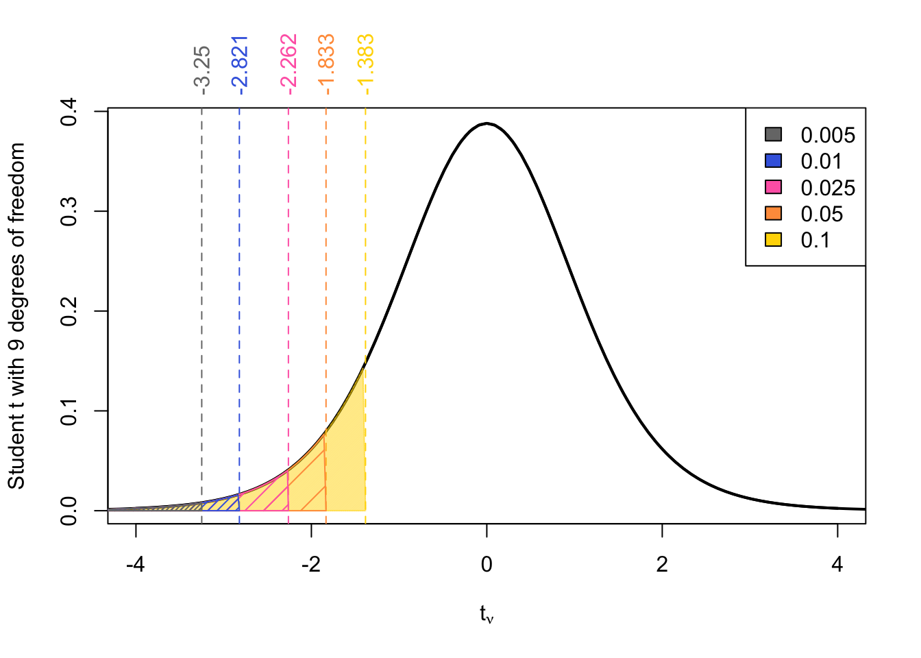
• If \(t_{\text{obs}}\) falls between two reference values in the row → the \(p\)-value falls between the corresponding probabilities shown at the top of the columns.
• If \(t_{\text{obs}}\) is greater than all negative reference values in the row → the \(p\)-value is greater than the largest probability listed (0.10).
• If \(t_{\text{obs}}\) is smaller than all negative reference values → the \(p\)-value is smaller than the smallest probability listed (0.050)

For two-tailed \(p\)-values

Important

Since a two-tailed \(p\)-value includes both tails of the distribution, we double the corresponding one-tailed probability to account for the symmetry of the \(t\)-distribution.

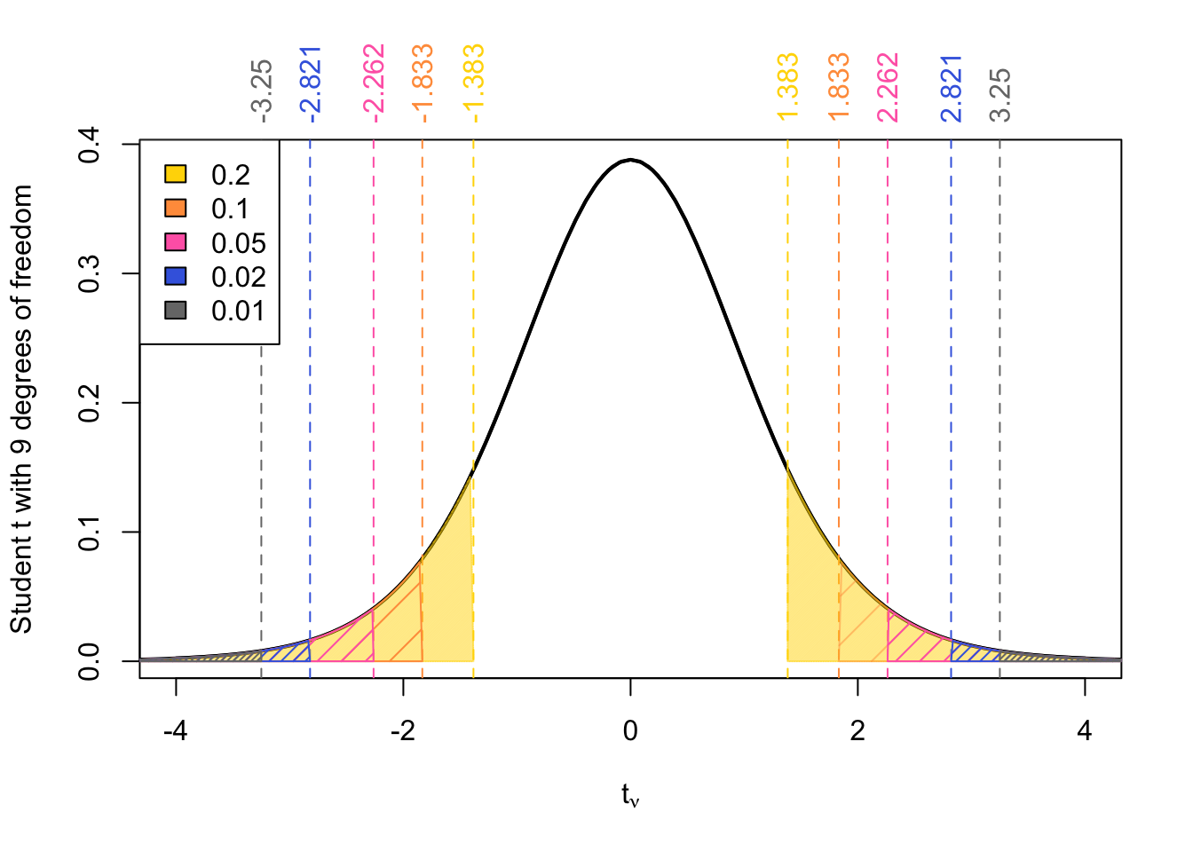
1. First, take the absolute value of your test statistic: \(|t_{\text{obs}}|\).

2. Compare \(|t_{\text{obs}}|\) to the positive reference values listed in the table.

3. Now determine where \(|t_{\text{obs}}|\) falls:

• If \(|t_\text{obs}|\) falls between two reference values → the \(p\)-value falls between the corresponding two-tailed probabilities (i.e., twice the one-tailed probabilities shown at the top of the columns).

• If \(|t_\text{obs}|\) is greater than all reference values → the \(p\)-value is less than twice the smallest probability listed (e.g., less than 0.01).

• If \(|t_\text{obs}|\) is smaller than all reference values → the \(p\)-value is greater than twice the largest probability listed (e.g., greater than 0.2).

Computing exact \(p\)-values

In R we can of course compute the exact \(p\)-values using the pt() function.

Lower-tailed \(p\)-values

pt(t_obs, df, lower.tail = FALSE)

Upper-tailed \(p\)-values

pt(t_obs, df, lower.tail = FALSE)

Two-tailed \(p\)-values

2 * pt(abs(t_obs), df, lower.tail = FALSE)

Examples

Upper-tailed test

For upper-tailed tests involving the null distribution \(t_{\nu}\), that is a Student \(t\)-distribution with \(\nu\) degrees of freedom, the \(p\)-value can be calculated as:

\[\begin{align} p\text{-value} &= \Pr(t_{obs} > t_{\nu}) \end{align}\]

where \(t_{obs}\) is our observed test statistic.

Example 1 Given a \(t_{obs}\) = 1 degrees of freedom \(\nu\) = 9

Solution

The reference row from the \(t\)-table is:

Given a \(t_{obs}\) = 1 degrees of freedom \(\nu\) = 9 the \(p\)-value can be approximated as:

\[\begin{align} p\text{-value} &= \Pr(t_{9} > t_\text{obs} ) \\ &= \Pr(t_{9} > 1)\\ &> \Pr(t_{9} > \textcolor{gold}{1.383}) = \textcolor{gold}{0.1} \end{align}\]

The exact \(p\)-value is found using:

pt(1, df = 9, lower.tail = FALSE)

[1] 0.1717182

The relationship between the exact \(p\)-value and the relant reference \(t\)-values is shown below. As we can see,

\[ p\text{-value} = 0.1717 > 0.1 \]

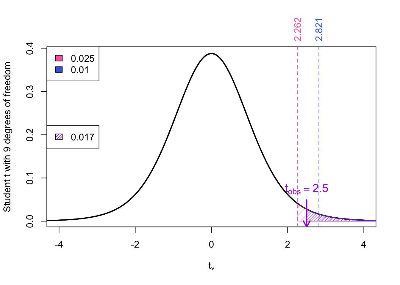
Example 2 Given a \(t_{obs}\) = 2.5 degrees of freedom \(\nu\) = 9

Solution

The reference row from the \(t\)-table is:

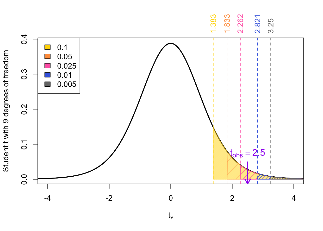
Given a \(t_{obs}\) = 2.5 degrees of freedom \(\nu\) = 9 the \(p\)-value can be approximated as:

\[ \begin{align} p\text{-value} &= \Pr(t_{9} > t_\text{obs} ) \\ &= \Pr(t_{9} > 2.5)\\ \implies \Pr(t_{9} > \textcolor{RoyalBlue}{2.821}) &< \Pr(t_{9} > 2.5) < \ \Pr(t_{9} > \textcolor{Magenta}{2.262}) \\ \textcolor{RoyalBlue}{0.01} &< \Pr(t_{9} > 2.5) < \ \textcolor{Magenta}{0.025} \end{align} \]

The exact \(p\)-value is found using:

pt(2.5, df = 9, lower.tail = FALSE)

[1] 0.01693091

The relationship between the exact \(p\)-value and the relant reference \(t\)-values is shown below. As we can see,

\[ \textcolor{RoyalBlue}{0.01} < p\text{-value} = 0.0169 < \textcolor{Magenta}{0.025} \]

Example 3 Given a \(t_{obs}\) = 5 degrees of freedom \(\nu\) = 9

Solution

The reference row from the \(t\)-table is:

Given a \(t_{obs}\) = 5 degrees of freedom \(\nu\) = 9 the \(p\)-value can be approximated as:

\[ \begin{align} p\text{-value} &= \Pr(t_{9} > t_\text{obs} ) \\ &= \Pr(t_{9} > 5) \\ & < \Pr(t_{9} > \textcolor{gray}{3.25}) = \textcolor{gray}{0.005} \\ \implies p\text{-value} &< \textcolor{gray}{0.005} \end{align} \]

The exact \(p\)-value is found using:

pt(5, df = 9, lower.tail = FALSE)

[1] 0.000369484

The relationship between the exact \(p\)-value and the relant reference \(t\)-values is shown below. As we can see,

\[ p\text{-value} = 4\times 10^{-4} < \textcolor{gray}{0.005} \]

Lower-tail tests

For lower-tailed tests involving the null distribution \(t_{\nu}\), that is a Student \(t\)-distribution with \(\nu\) degrees of freedom, the \(p\)-value can be calculated as:

\[\begin{align} p\text{-value} &= \Pr(t_{obs} < t_{\nu}) \end{align}\]

where \(t_{obs}\) is our observed test statistic.

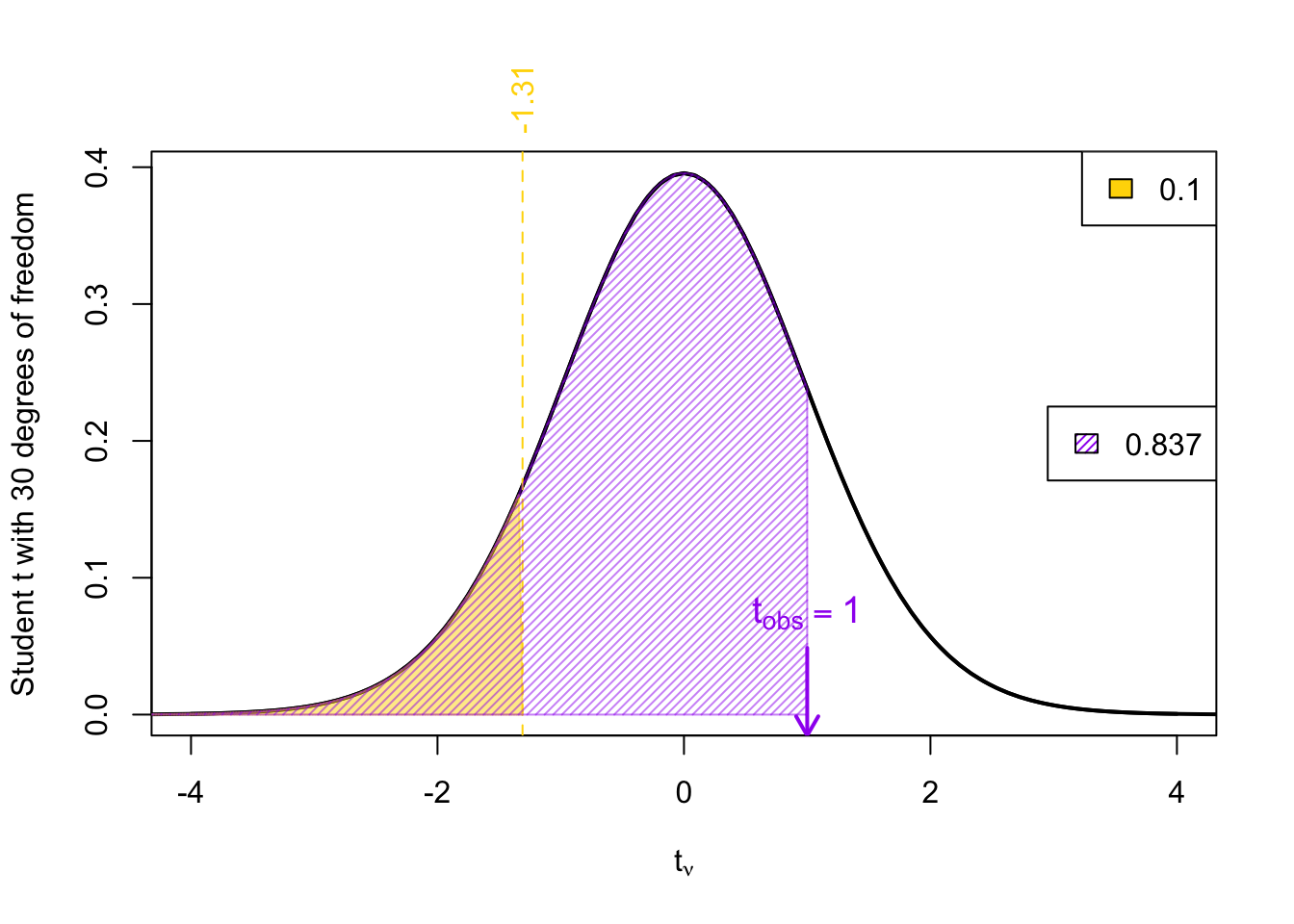
Example 4 Given a \(t_{obs}\) = 1 degrees of freedom \(\nu\) = 30

Solution

The reference row from the \(t\)-table is:

Given a \(t_{obs}\) = 1 degrees of freedom \(\nu\) = 30 the \(p\)-value can be approximated as:

\[\begin{align} p\text{-value} &= \Pr(t_{30} < t_\text{obs} ) \\ &= \Pr(t_{30} < 1)\\ &> \Pr(t_{30} < \textcolor{gold}{-1.31}) = \textcolor{gold}{0.1} \end{align}\]

The exact \(p\)-value is found using:

pt(1, df = 30, lower.tail = TRUE)
pt(1, df = 30) # same as above

[1] 0.8373457

The relationship between the exact \(p\)-value and the relant reference \(t\)-values is shown below. As we can see,

\[ p\text{-value} = 0.8373 > 0.1 \]

Example 5 Given a \(t_{obs}\) = -1.5 degrees of freedom \(\nu\) = 30

Solution

The reference row from the \(t\)-table is:

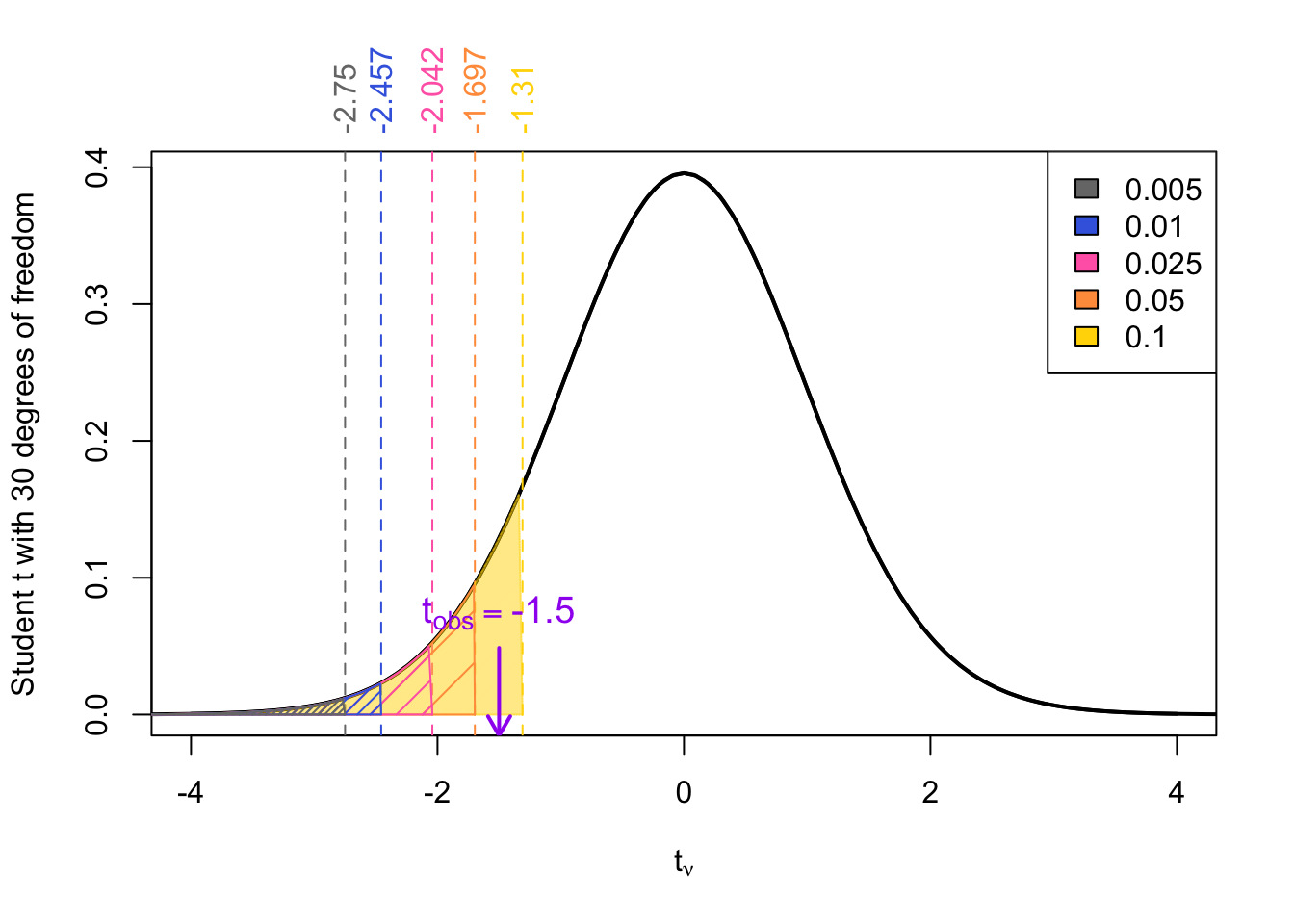
Given a \(t_{obs}\) = -1.5 degrees of freedom \(\nu\) = 30 the \(p\)-value can be approximated as:

\[ \begin{align} p\text{-value} &= \Pr(t_{30} < t_\text{obs} ) \\ &= \Pr(t_{30} < -1.5)\\ \implies \Pr(t_{30} <\textcolor{orange}{-1.697}) &< \Pr(t_{30}< 1.5) < \ \Pr(t_{30} < \textcolor{gold}{-1.31}) \\ \textcolor{orange}{0.05} &< \Pr(t_{30} < 1.5)< \ \textcolor{gold}{0.1} \end{align} \]

The exact \(p\)-value is found using:

pt(-1.5, df = 30, lower.tail = TRUE)
pt(-1.5, df = 30) # same as above

[1] 0.07203296

The relationship between the exact \(p\)-value and the relant reference \(t\)-values is shown below. As we can see,

\[ \textcolor{orange}{0.05} < p\text{-value} = 0.072 < \textcolor{gold}{0.1} \]

Given a \(t_{obs}\) = -3.2 degrees of freedom \(\nu\) = 30

Solution

The reference row from the \(t\)-table is:

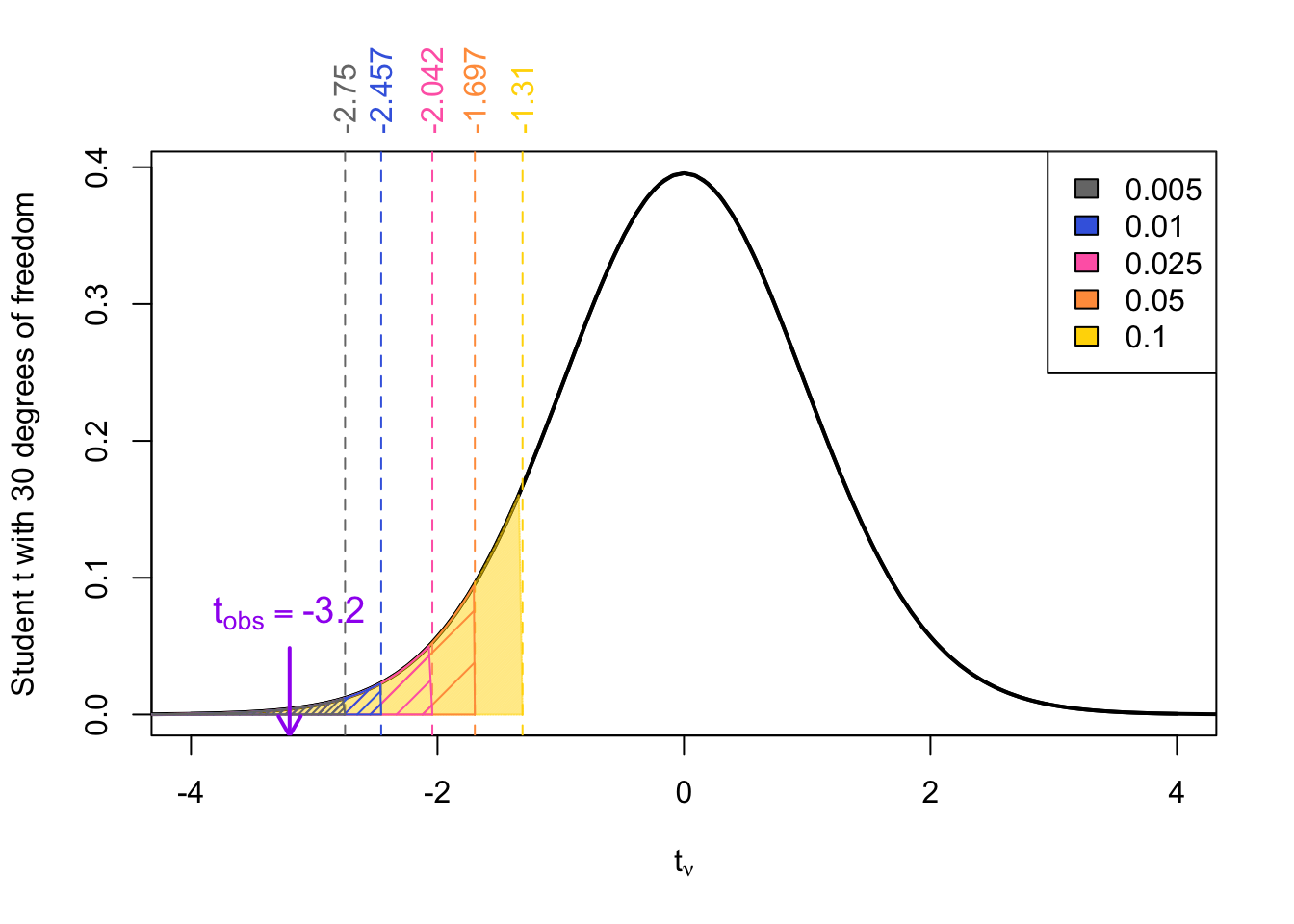
Given a \(t_{obs}\) = -3.2 degrees of freedom \(\nu\) = 30 the \(p\)-value can be approximated as:

\[ \begin{align} p\text{-value} &= \Pr(t_{30} < t_\text{obs} ) \\ &= \Pr(t_{30} < -3.2) \\ & < \Pr(t_{30} < \textcolor{gray}{-2.75}) = \textcolor{gray}{0.005} \\ \implies p\text{-value} &< \textcolor{gray}{0.005} \end{align} \]

The exact \(p\)-value is found using:

pt(-3.2, df = 30, lower.tail = TRUE)
pt(-3.2, df = 30) # same as above 

[1] 0.001619301

The relationship between the exact \(p\)-value and the relant reference \(t\)-values is shown below. As we can see,

\[ p\text{-value} = 0.0016 < \textcolor{gray}{0.005} \]

Two-tailed tests

For two-tailed tests involving the null distribution \(t_{\nu}\), that is a Student \(t\)-distribution with \(\nu\) degrees of freedom, the \(p\)-value can be calculated as:

\[\begin{align} p\text{-value} &= 2 \times \Pr(t_{obs} < | t_{\nu}| ) \end{align}\]

where \(t_{obs}\) is our observed test statistic.

Example 6 Given a \(t_{obs}\) = 1 degrees of freedom \(\nu\) = 15

Solution

The reference row from the \(t\)-table is:

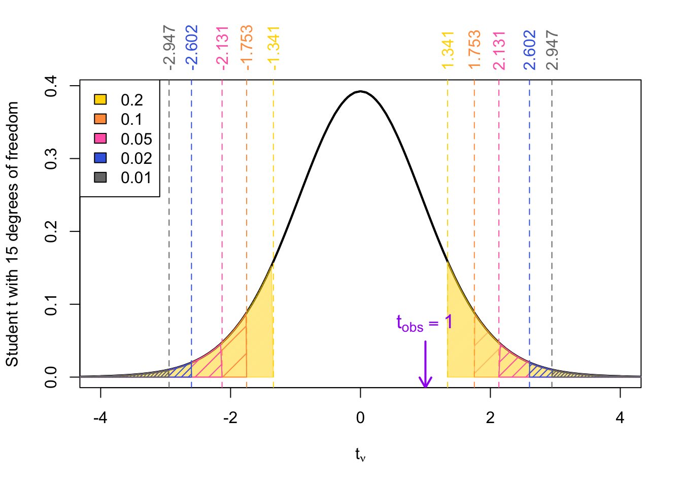
Given a \(t_{obs}\) = 1 degrees of freedom \(\nu\) = 15 the \(p\)-value can be approximated as:

\[\begin{align} p\text{-value} &= 2 \times \Pr(t_{15} > |t_\text{obs}| ) \\ &= 2 \times \Pr(t_{15} > 1)\\ &> 2 \times \Pr(t_{15} < \textcolor{gold}{1.341}) = 2 \times \textcolor{gold}{0.1}\\ \implies p\text{-value} &> 0.2 \end{align}\]

The exact \(p\)-value is found using:

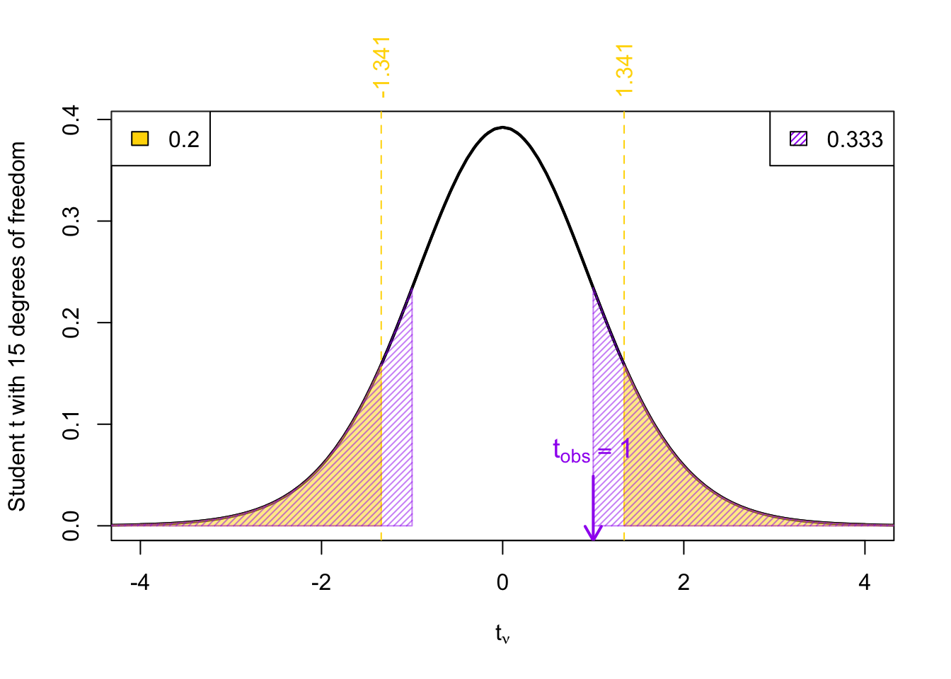
2 * pt(abs(1), df = 15, lower.tail = FALSE)

[1] 0.3331701

The relationship between the exact \(p\)-value and the relant reference \(t\)-values is shown below. As we can see,

\[ p\text{-value} = 0.3332 > 0.1 \]

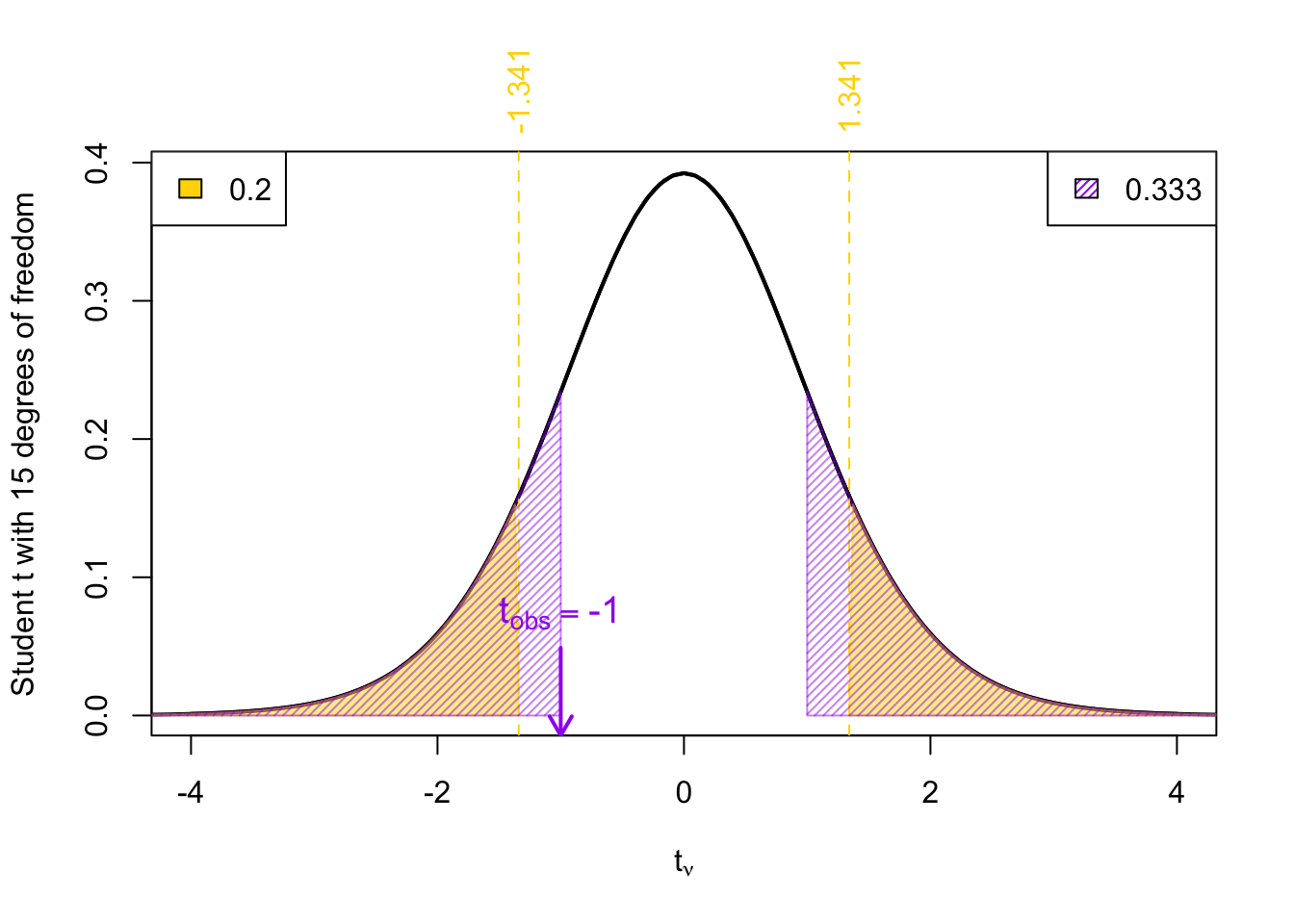
Given a \(t_{obs}\) = -1 degrees of freedom \(\nu\) = 15

Solution

Since the two-tailed \(p\)-value is defined as:

\[ p\text{-value} = 2 \times \Pr(t_{obs} < | t_{\nu}|) \]

the two-tailed \(p\)-value associated with \(t_\text{obs}\) = -1 will be the same as the two-tailed \(p\)-value associated with \(t_\text{obs}\) = 1.

The reference row from the \(t\)-table is:

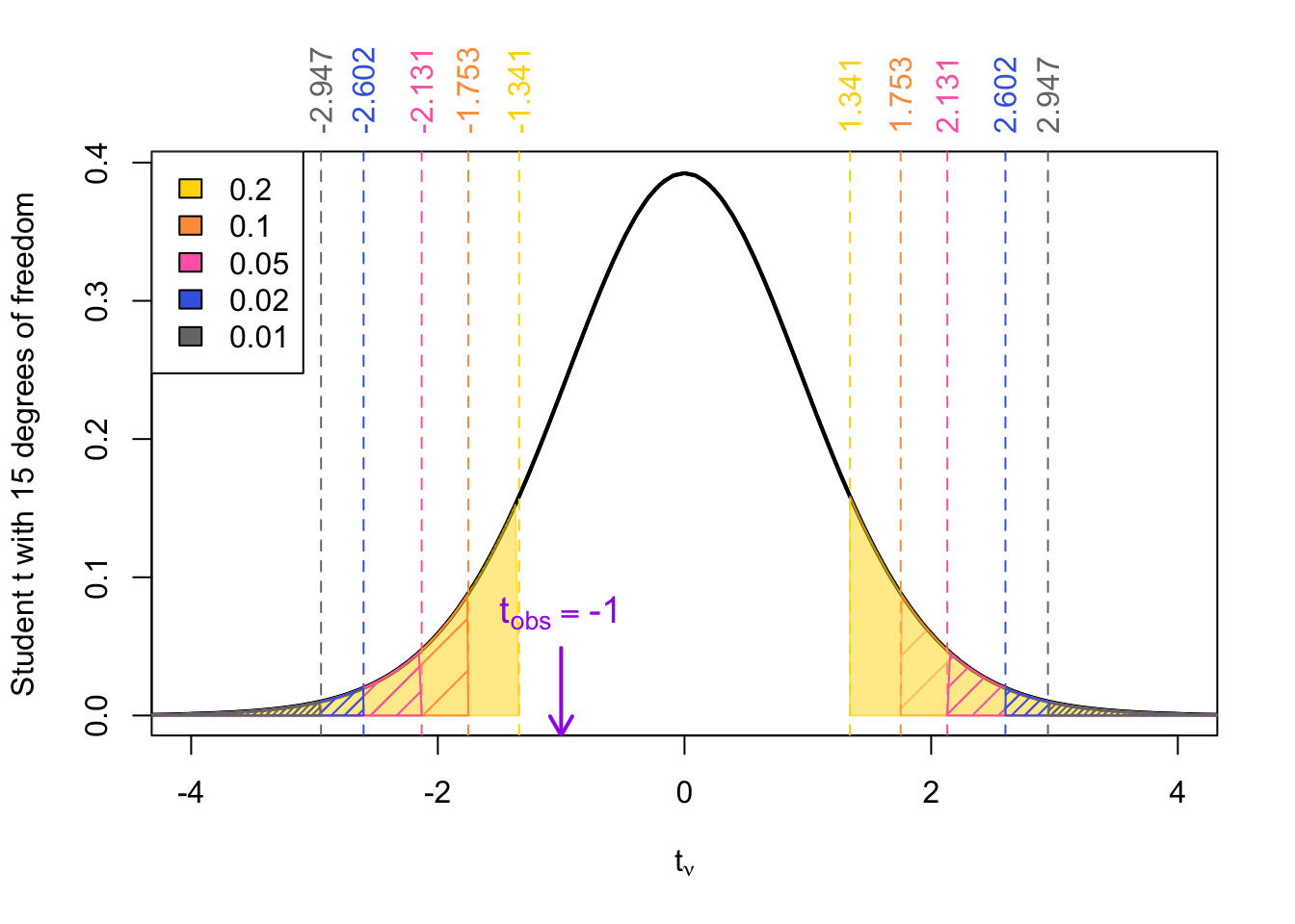
Given a \(t_{obs}\) = -1 degrees of freedom \(\nu\) = 15 the \(p\)-value can be approximated as:

\[\begin{align} p\text{-value} &= 2 \times \Pr(t_{15} > |t_\text{obs}| ) \\ &= 2 \times \Pr(t_{15} > 1)\\ &> 2 \times \Pr(t_{15} < \textcolor{gold}{1.341}) = 2 \times \textcolor{gold}{0.1}\\ \implies p\text{-value} &> 0.2 \end{align}\]

The exact \(p\)-value is found using:

2 * pt(abs(-1), df = 15, lower.tail = FALSE)

[1] 0.3331701

The relationship between the exact \(p\)-value and the relant reference \(t\)-values is shown below. As we can see,

\[ p\text{-value} = 0.3332 > 0.1 \]

Example 7 Given a \(t_{obs}\) = -1.5 degrees of freedom \(\nu\) = 15

Solution

The reference row from the \(t\)-table is:

Given a \(t_{obs}\) = -1.5 degrees of freedom \(\nu\) = 15 the \(p\)-value can be approximated as:

\[ \begin{align} p\text{-value} &= 2 \times \Pr(t_{15} > | t_\text{obs} | ) \\ &= 2 \times \Pr(t_{15} > |-1.5|)\\ &= 2 \times \Pr(t_{15} > 1.5) \end{align} \] And since \[ \begin{align} \Pr(t_{15} > \textcolor{orange}{-1.753}) &< \Pr(t_{15} > 1.5) < \ \Pr(t_{15} > \textcolor{gold}{-1.341}) \\ \implies 2 \times \Pr(t_{15} > \textcolor{orange}{-1.753}) &< 2 \times \Pr(t_{15} > 1.5) < \ 2 \times \Pr(t_{15} > \textcolor{gold}{-1.341}) \\ 2 \times\textcolor{orange}{0.05} &< 2 \times \Pr(t_{15} < 1.5) > \ 2 \times \textcolor{gold}{0.1} \\ \ 0.1 &< p\text{-value} < 0.2 \end{align} \]

Example 8 Find the two-sided \(p\)-value for \(t_{\text{obs}} = -3.5\) with \(\nu =15\) degrees of freedom.

Solution

The reference row from the \(t\)-table is:

Given a \(t_{obs}\) = -3.5 degrees of freedom \(\nu\) = 15 the \(p\)-value can be approximated as:

\[ \begin{align} p\text{-value} &= 2 \times \Pr(t_{15} > t_\text{obs} ) \\ &= 2 \times \Pr(t_{15} > -3.5) \\ & < 2 \times \Pr(t_{15} > \textcolor{gray}{2.947}) = 2 \times \textcolor{gray}{0.005} \\ \implies p\text{-value} &< \textcolor{gray}{0.01} \end{align} \]

The exact \(p\)-value is found using:

2*pt(abs(-3.5), df = 15, lower.tail = FALSE)

[1] 0.003223531

The relationship between the exact \(p\)-value and the relant reference \(t\)-values is shown below. As we can see,

\[ p\text{-value} = 0.0032 < \textcolor{gray}{0.005} \]