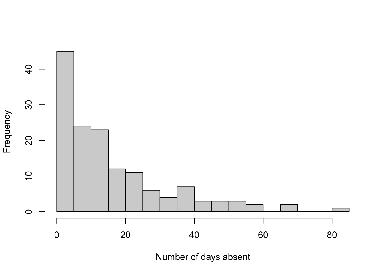
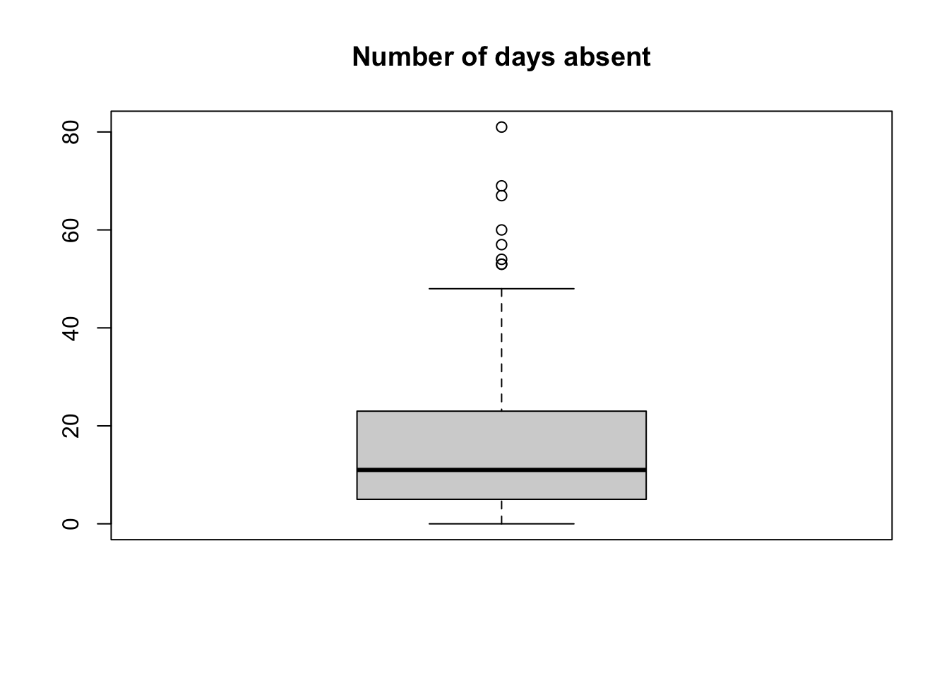
round(median(absenteeism$days),2)[1] 11STAT 205: Introduction to Mathematical Statistics
Exercise 1.1 What is the extension for quarto documents?
.rmd.qmd.html.r.qrtExercise 1.2 What does echo: false do in a Quarto code chunk?
Exercise 1.3 Which of the following is NOT part of the YAML section in a Quarto document?
titleauthoroutputsubtitleExercise 1.4 What is the syntax for producing code chunks in Quarto?
r inside{r} at the start:{r} inside{.r} at the start:Exercise 1.5 What does echo: false do in a Quarto code chunk?
Exercise 1.6 Why is setting a seed important in R, and how do you set one?
Exercise 1.7 Based on the output below, identify which data type x has been coded as.
x <- factor(c("A", "B", "C", "A"),
        levels = c("A", "B", "C"))
xExercise 1.8 In the context of variables, which of the following is an example of a categorical variable?
Exercise 1.9 Which measure of central tendency is defined as the middle value when data is ordered?
Exercise 1.10 The Interquartile Range (IQR) measures:
Exercise 1.11 What does the breaks argument in the hist function do?
Exercise 1.12 Consider Figure Figure 1.1, estimate the median number of absent days.
Exercise 1.13 What is the primary difference between descriptive and inferential statistics?
Exercise 1.14 In the context of sampling methods, what is a simple random sample?
Exercise 1.15 Explain what selection bias is and provide an example of how it might occur in a research study.
Exercise 1.16 Which type of study involves observing individuals or groups and collecting data without intervening or manipulating any aspect of the study participants?
Exercise 1.17 Suppose a researcher wants to study the average income of households in Kelowna.
Exercise 2.1 Which of the following statements best describes statistics?
Exercise 2.2 True or False: Parameters are descriptive measures computed from a sample, while statistics are descriptive measures computed from a population.
Exercise 2.3 Let \(X_1,\dots, X_n\) be a random sample from a gamma probability distribution with parameters \(\alpha\) and \(\beta\).
Recall the Probability Density Function (PDF) of the Gamma Distribution:
\[ f(x; \alpha, \beta) = \frac{\beta^\alpha x^{\alpha - 1} e^{-\beta x}}{\Gamma(\alpha)} \]
where \(x > 0\), \(\alpha > 0\) is the shape parameter, \(\beta > 0\) is the rate parameter, and \(\Gamma(\alpha) = \int_0^\infty x^{\alpha - 1} e^{-x} \, dx\) is the gamma function. Find the method of moment (MoM) estimators for the unknown parameters \(\alpha\) and \(\beta\). You may use the results below:
\[\begin{align} \mathbb{E}[X] &= \alpha\beta, & \text{Var}(X) &= \alpha\beta^2 \end{align}\]
Exercise 2.4 Which of the following best describes the concept of sampling distribution?
Exercise 2.5 Let \(X_1, \dots, X_n\) be \(N(\mu, \sigma^2)\).
Exercise 2.6 Let \(\hat{\theta}_1\) be the sample mean and \(\hat{\theta}_2\) be the sample median. It is known that
\[ \text{Var}(\hat{\theta}_2) = (1.2533)^2 \frac{\sigma^2}{n} \]
Find the efficiency of \(\hat{\theta}_2\) relative to \(\hat{\theta}_1\).
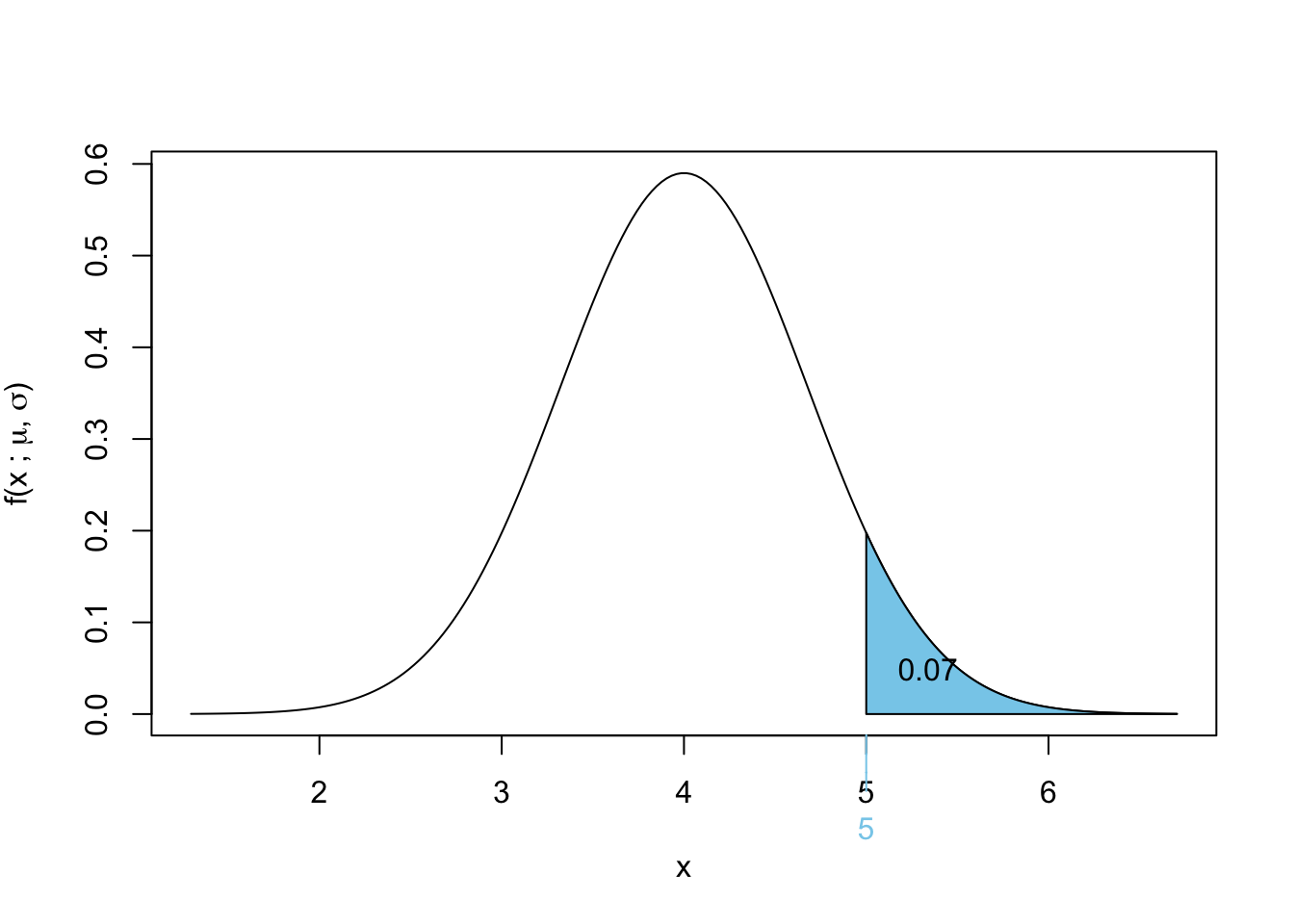
Exercise 2.7 Suppose we have a manufacturing process where widgets are produced, and the time it takes for a widget to be completed follows an exponential distribution with a mean time of 4 hours. If thirty-five widgets from this manufacturer are chosen at random:
We compute:
\[ \Pr(\bar{X} > 5) = \Pr \left( Z > \frac{5 - \mu_{\bar{X}}}{\sigma_{\bar{X}}} \right) \]
Substituting values:
\[ \Pr \left( Z > \frac{5 - 4}{4/\sqrt{35}} \right) \]
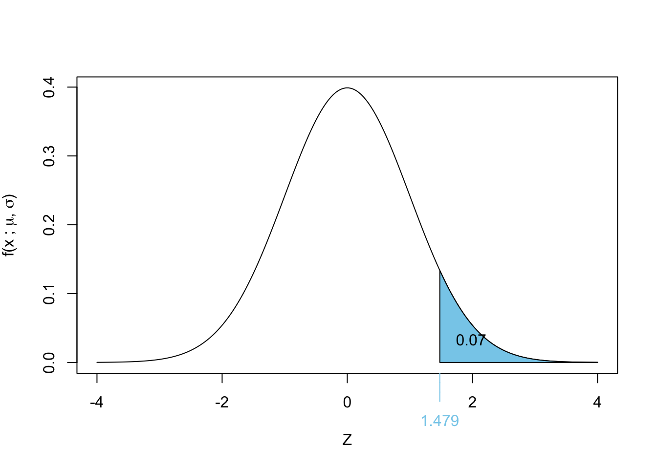
\[ = \Pr(Z > 1.4790199) \]
Using standard normal tables:
\[\begin{align*} \Pr(Z > 1.479) &= 1 - \Pr(Z \leq 1.479)\\ &= 1 - \Pr(Z \leq 1.479)\\ &= 1 - 0.9304\\ &\approx 0.0696\\ \end{align*}\]
Thus, the probability that the mean failure time exceeds 5 hours is 0.0696.
A graphical representation is shown below:
Exercise 2.8 Let \(X_1, X_2, \dots, X_5\) be a random sample from a normal distribution with mean 55 and variance 223. Let
\[ Y = \sum_{i=1}^{5} \frac{(X_i - \bar{X})^2}{223} \]
\[\begin{align*}
\Pr(Y \leq 2)
&= \Pr(\chi^2_4 \leq 2) \\
&= 1 - \Pr(\chi^2_4 \geq 2) \\
&= 1 - 0.2642411 \\
&= 0.2642411
\end{align*}\]

How would you calculate this probability in R?
pchisq(2, df = n-1, lower.tail = FALSE)qchisq(2, df = n-1, lower.tail = FALSE)pchisq(2, df = n-1)pchisq(1-2, df = n-1)pchisq(a, df = n-1) # option C[1] 0.2642411Incorrect answers (wrong tail/ wrong function/ wrong quantile)
pchisq(a, df = n-1, lower.tail = FALSE)  # option A
qchisq(a, df = n-1, lower.tail = FALSE)  # option B
Warning in qchisq(a, df = n - 1, lower.tail = FALSE): NaNs producedpchisq(1-a, df = n-1) # option D[1] 0.7357589
[1] NaN
[1] 0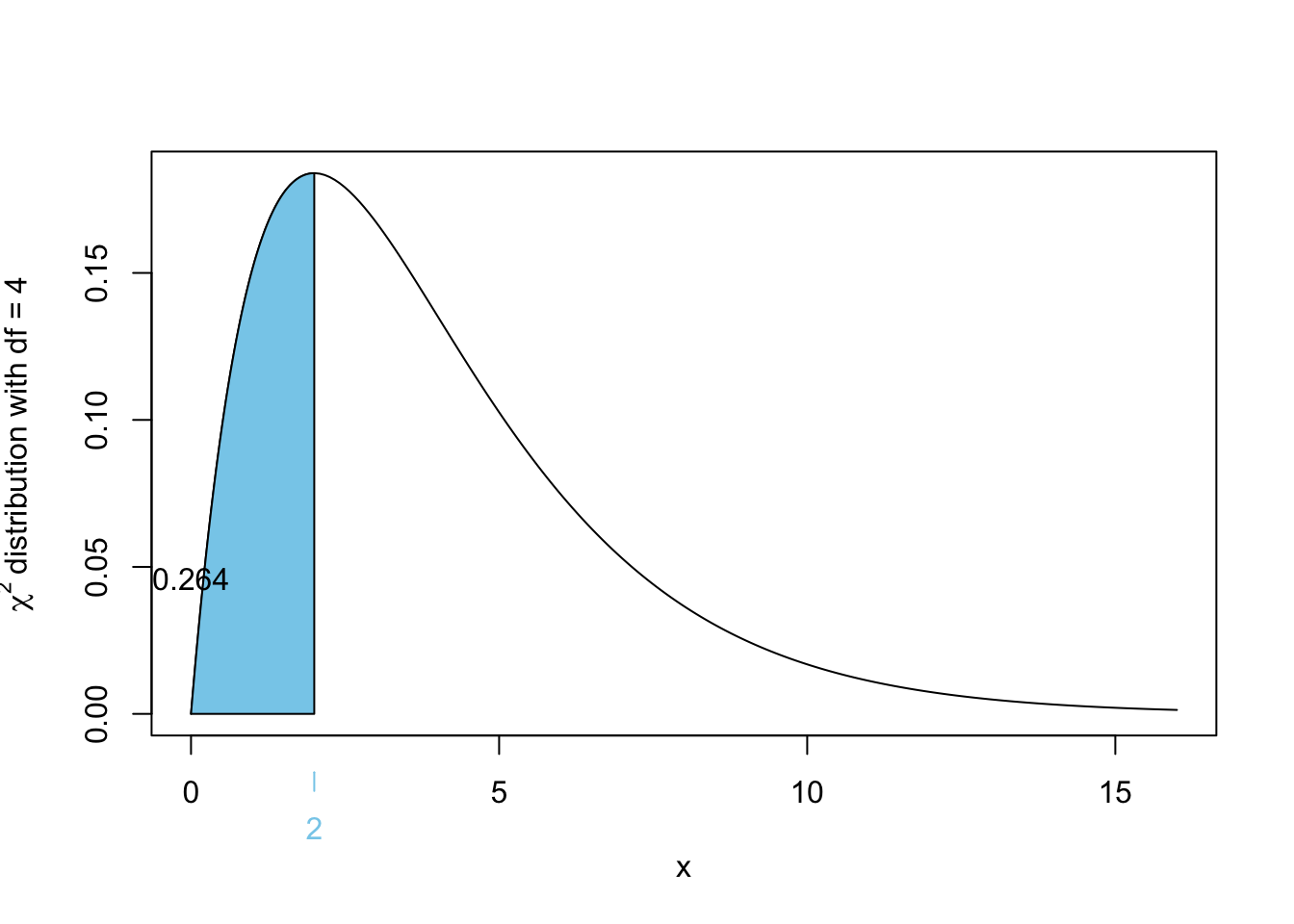
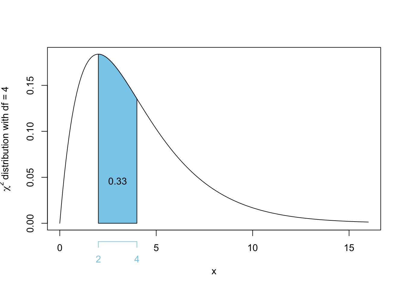
\[\begin{align*}
\Pr(2 \leq Y \leq 4)
&= \Pr(Y \leq 4) - \Pr(Y \leq 2) \\
&= \Pr(\chi^2_4 \leq 4) - \Pr(\chi^2_4 \leq 2) \\
&= \Pr(\chi^2_4 \geq 2) - \Pr(\chi^2_4 \geq 4) \\
&= 0.7357589 - 0.4060058\\
&= 0.329753 \approx 0.33
\end{align*}\]
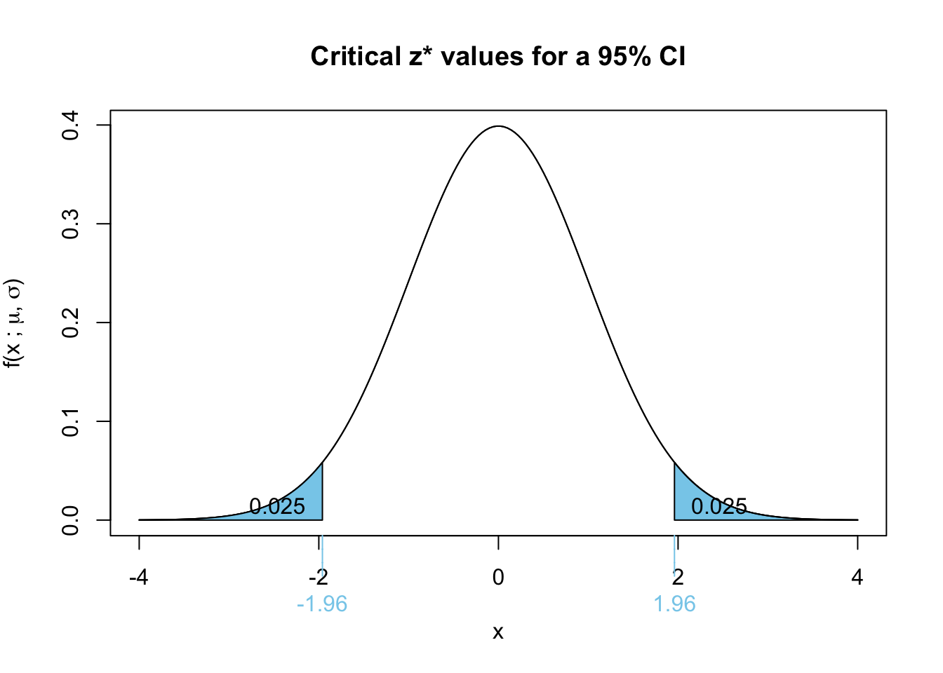
Exercise 3.1 Which of the following best describes the purpose of a confidence interval?
Exercise 3.2 As part of an investigation from Union Carbide Corporation, the following data represent naturally occurring amounts of sulfate S04 (in parts per million) in well water. The data is from a random sample of 24 water wells in Northwest Texas.
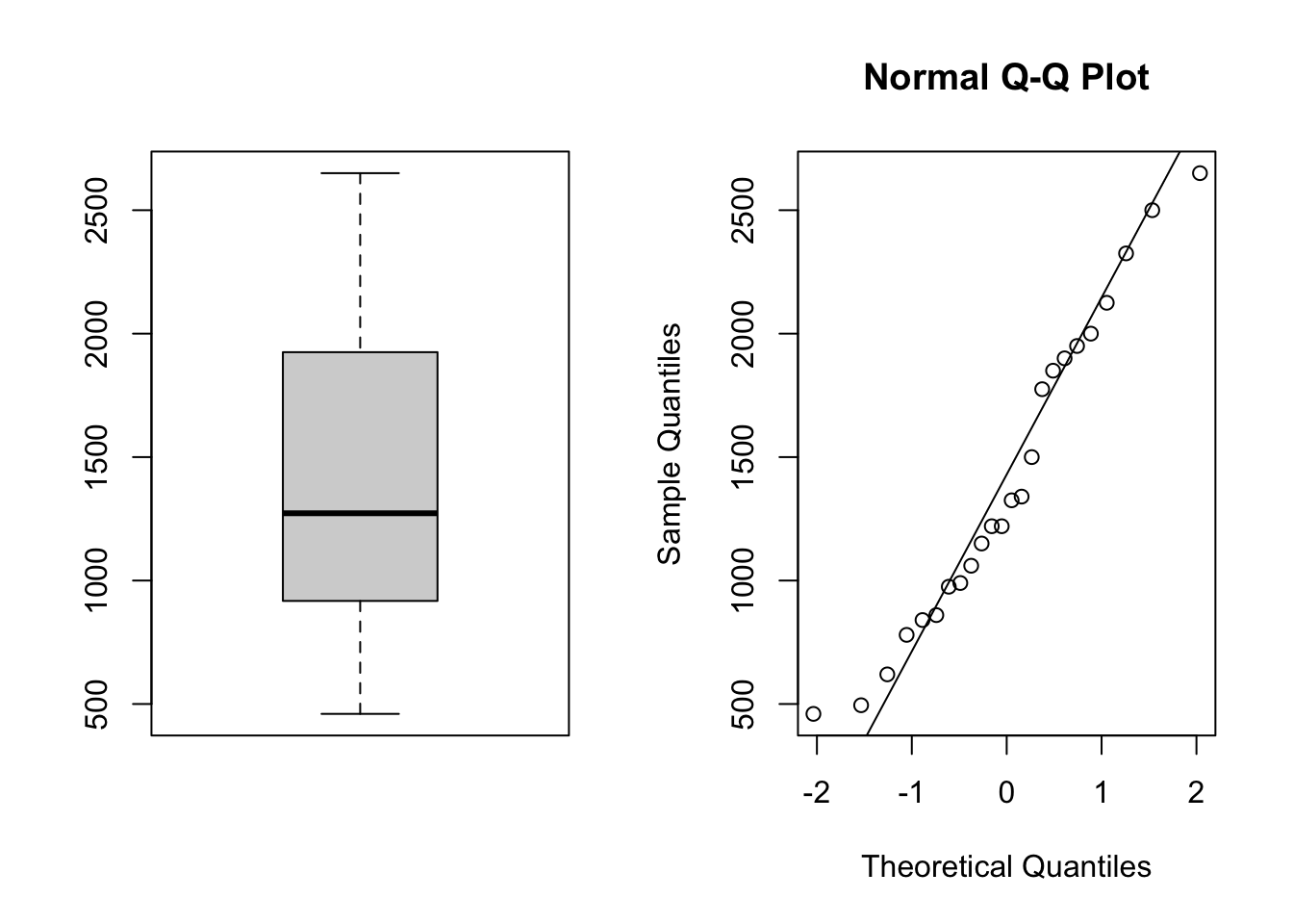
Based on the following summary statistics, estimate the standard error for \(\bar{X}\) (assume that the 24 observations are stored in a vector called data)
c(mean(data), median(data), sd(data), var(data))[1] 1412.9167 1272.5000 636.4592 405080.2536Exercise 3.3 In New York City on October 23rd, 2014, a doctor who had recently been treating Ebola patients in Guinea went to the hospital with a slight fever and was subsequently diagnosed with Ebola. Soon thereafter, an NBC 4 New York/The Wall Street Journal/Marist Poll found that 82% of New Yorkers favored a “mandatory 21-day quarantine for anyone who has come into contact with an Ebola patient.” This poll included responses from 1042 New York adults between October 26th and 28th, 2014.
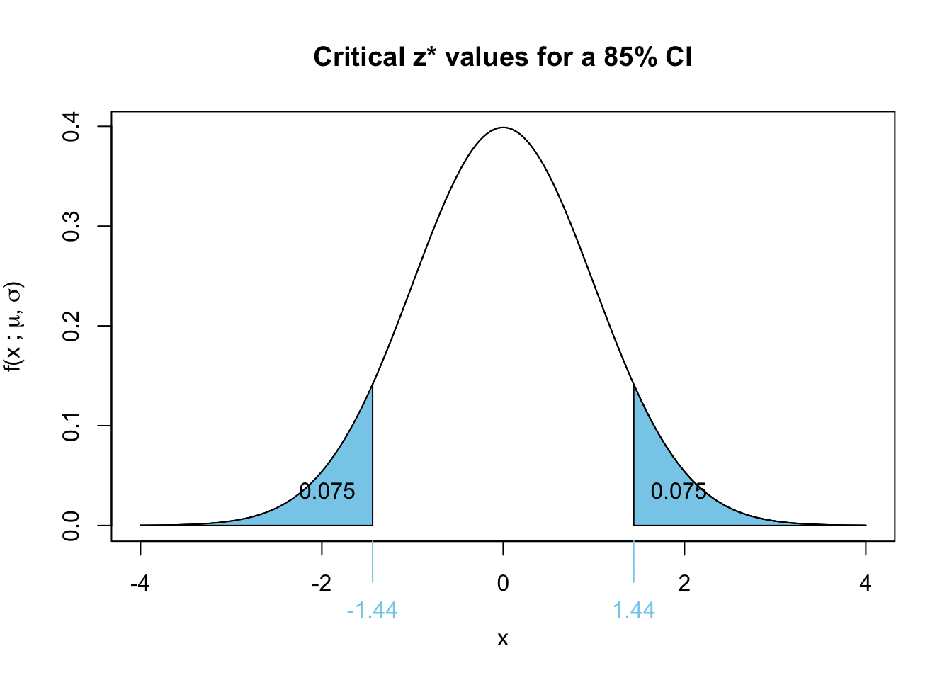
narrower
A lower confidence level corresponds to a smaller \(z^*\) value, which results in a narrower confidence interval.