
Midterm 2 Review
STAT 205: Introduction to Mathematical Statistics
Information
Coverage: Lectures 6 - 13 inclusive, Assignments 3 and 4.
Allowable materials:
One page (letter-sizes) two-sided cheat sheet
- I encourage you to handwrite your cheatsheet
- You will be required to hand this in at the end of the test. I encourage you to make a copy if you would like to keep it for the exam.
Non-graphing, non-programmable calculator (e.g. Casio FX-991, Sharp EL-W516, EL-520 , Texas Instruments TI-36X Pro, CASIO fx-991ES PLUS C*). If you are unsure if your calculator is permitted, please ask me ASAP.
Format
The midterm closed book. The general structure will be as follows:
- Multiple choice,
- True/False (with supporting statements required),
- Short Answer (2-3 sentences concept questions) and
- Long Answer (working through examples with multiple parts)
Material provided:
- Standard Normal Table
- Student t-Distribution
- Chi-squared distribution table (you won’t need this table for this midterm but I want to reuse the tables from midterm 1)
- Partial R help documents (e.g. ?t-test(), ?dt(); see stat205-exam.pdfDownload stat205-exam.pdfpage 2 for example)
Practice Problem (in order of usefulness):
Some practice problems have been uploaded to Canvas to provide examples of structure and difficulty level.
- Assignment questions
- Suggested problems in https://irene.vrbik.ok.ubc.ca/quarto/stat205/#tentative-schedule
- Past midterm and exam (see Canvas)
Topics
This midterm covers Lectures 6 to 13 inclusively which generally deals with Statistical Inference. The main types of statistical inference can be broadly categorized into two approaches:
Estimation
Point Estimation
Provides a single numeric value (estimator) to estimate a population parameter. Example: Sample mean (\(\bar{x}\)) estimates population mean (\(\mu\)).Confidence Interval Estimation
Provides a range of plausible values likely containing the true parameter. Example: Confidence intervals.
Hypothesis Testing
Unless other specified we use a significance level (\(\alpha\)) of 0.05. Steps:
- Check assumptions
- State null (\(H_0\)) and alternative hypotheses (\(H_a\)).
- Compute test statistic.
- Make decision based on critical values or \(p\)-values.
- State the conclusion.
Hypothesis Testing
Hypothesis testing is a statistical method used to make inferences about a population parameter based on sample data. It involves setting up two competing hypotheses, the null hypothesis (\(H_0\)) and the alternative hypothesis (\(H_A\)), and testing whether the evidence from the sample supports rejecting the null hypothesis in favor of the alternative hypothesis.
Unless other specified we use a significance level of 5% (i.e. assume \(\alpha = 0.05\) unless otherwise specified). A summary of the types of tests we have talked about are summarized below:
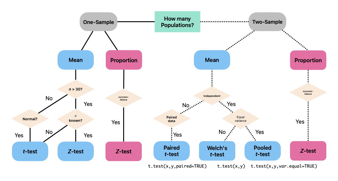
Here are the basic steps involved in hypothesis testing:
0. Check the Assumptions
Required for all of our tests:
- Ensure data are collected through random sampling or randomized experiments.
- Confirm independence of observations.
Require for some tests (see Figure 1):
- Verify normality of the underlying population or assess sample size adequacy for normal approximation (via Central Limit Theorem).
- For proportions, confirm sample sizes are sufficient for using normal approximations (e.g., \(np \geq 10\) and \(n(1 - p) \geq 10\)).
- For comparisons between groups, check equality of variances if relevant (e.g., for pooled two-sample t-tests).
1. State the Hypotheses:
- Null Hypothesis (\(H_0\)): Represents the default assumption, often stating that there is no effect or no difference (i.e. no-change or status-quo).
- Alternative Hypothesis(\(H_A\)): Represents the claim or research question you are testing for, stating that there is an effect or a difference.
2. Test Statistic
- Identify the appropriate null distribution1; that is, determine the distribution of the test statistic assuming \(H_0\) is true.
- Calculate the appropriate test statistic based on the chosen test and the sample data.
3. Decision (Critical Value or p-value)
- Based on the assumed sampling distribution of the test statistic, calculate either the critical value or the \(p\)-value.
- Make a Decision: Clearly state your conclusion in terms of rejecting or failing to reject the null hypothesis (\(H_0\)).
- critical value approach: if the test statistic falls with the rejection region, reject \(H_0\) in favour of \(H_A\), otherwise, fail to reject \(H_0\).
- \(p\)-value approach: if the \(p\)-value is less than the significance level (\(\alpha\)), reject \(H_0\) in favour of \(H_A\), otherwise, fail to reject \(H_0\).
4. Conclusions
- Based on the decision in the previous step, draw conclusions about the population parameter(s) being tested.
- Interpret the results in the context of the research question or problem being investigated, explicitly referring to the alternative hypothesis (\(H_a\)).
- Avoid statements implying absolute certainty.
- Examples:
- There is sufficient evidence that the average exam scores differ between teaching methods.
- There is insufficient evidence to conclude that the drug reduces blood pressure.
Critical Value Approach
As it’s name suggests the critical value approach depends on the so-called critical value(s). These values define the so-called rejection region (as depicted in red in Figure 2) which comprise the set of values of the test statistic for which the null hypothesis is rejected. These boundaries are chosen based on:
- the chosen significance level (\(\alpha\)),
- the distribution of the test statistic under the null hypothesis, and
- the specification of the alternative hypothesis \(H_A\) (either two-tailed, lower-tailed, or upper-tailed).
If the observed test statistic falls within the rejection region, the \(H_0\) is rejected in favour of \(H_A\).
p-value approach
The \(p\)-value approach involves comparing a \(p\)-value with your significance level \(\alpha\) (unless otherwise speicified, assumed to be 0.05). The \(p\)-value is the probability of observing a test statistic as extreme as, or more extreme (in the direction of \(H_A\)) than the one obtained from the sample data. If the \(p\)-value is less than \(\alpha\), the null hypothesis is rejected in favour of the alternative hypothesis. Otherwise, we fail to reject \(H_0\).
A note on finding \(p\)-values using the t-tables
When finding \(p\)-values from the t-tables you will only be able to get approximate ranges.
🗒️ Step-by-Step Guide:
Compute Test Statistic
Your test statistic will have the form:
\[ \frac{\text{estimate} - \text{null/hypothesize value}}{\text{standard error of estimate}} \sim t_{\nu} \]
where \(\nu\) are the degrees of freedom of a Student \(t\) distribution.
Determine the degrees of freedom
The degrees of will depend on what \(t\)-tests you are doing:
One-sample t-test: \(\nu = n - 1\)
Paired t-test: \(\nu = n - 1\) where \(n\) is the number of paired observations
Pooled t-test (equal variance): \(\nu = n_1 + n_2 - 2\)
Welch procedure (unequal variance):
\[ \begin{align} \nu &= \frac{\left(\frac{s_1^2}{n_1} + \frac{s_2^2}{n_2}\right)^2}{\frac{\left(\frac{s_1^2}{n_1}\right)^2}{n_1 - 1} + \frac{\left(\frac{s_2^2}{n_2}\right)^2}{n_2 - 1}}\\ &> \min\{n_1 - 1, n_2 -1\} \\ \end{align} \]
Welch’s conservative degrees of freedomUsing the smaller of the two degrees of freedom ensures that the critical value from tables is slightly larger, resulting in a larger (conservative) p-value. Since the Welch’s formula can be cumbersome to compute by hand, you can use the simplified conservative calculation on paper exams.
Round down degrees of freedom (Conservative Approach)If the degrees of freedom you calculated are not listed exactly on the t-table, you may round down and use the next lowest value of degrees of freedom on your table.
If \(\nu = 37\), but your table lists only 36 and 38, we use \(\nu = 36\) as your conservative approximation..
If \(\nu = 50\), but your table lists only 38 and \(\infty\), we use \(\nu = 38\) as your conservative approximation..
Using the t-table to find the neighbouring t-values
- Go to the t-table
- Look for the row corresponding to your degrees of freedom on the (left-hand side of the table indicated by the rows).
- If your exact \(t_{obs}\) isn’t listed, find it’s neighbouring t-value(s).
Express your \(p\)-value as range
For one-sided tests, this will be of the form:
\[ \begin{align} & \ p-\text{value} < 0.005\\ 0.005 < & \ p-\text{value} < 0.01\\ 0.01 < & \ p-\text{value} < 0.025\\ 0.025 < & \ p-\text{value} < 0.05\\ 0.05 < & \ p-\text{value} < 0.10\\ & \ p-\text{value} > 0.10 \end{align} \]
For two-sided test, this will be of the form:
\[ \begin{align} & \ p-\text{value} < 0.01\\ 0.01 < & \ p-\text{value} < 0.02\\ 0.02 < & \ p-\text{value} < 0.05\\ 0.05 < & \ p-\text{value} < 0.10\\ 0.10 < & \ p-\text{value} < 0.20\\ & \ p-\text{value} > 0.20 \end{align} \]
Examples:
Suppose we had:
- Calculated t-value: 2.75
- Degrees of freedom: \(\nu = 5\)
Upper tail p-value
For a upper-tailed test, our reference values would be:
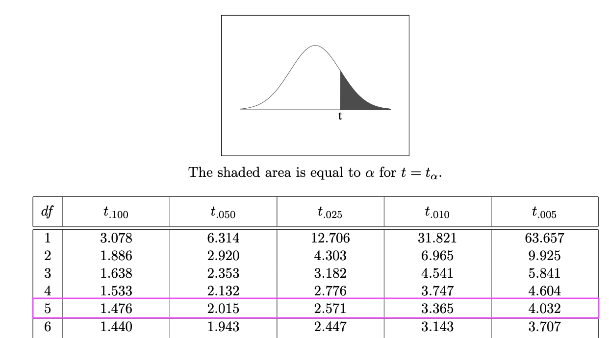
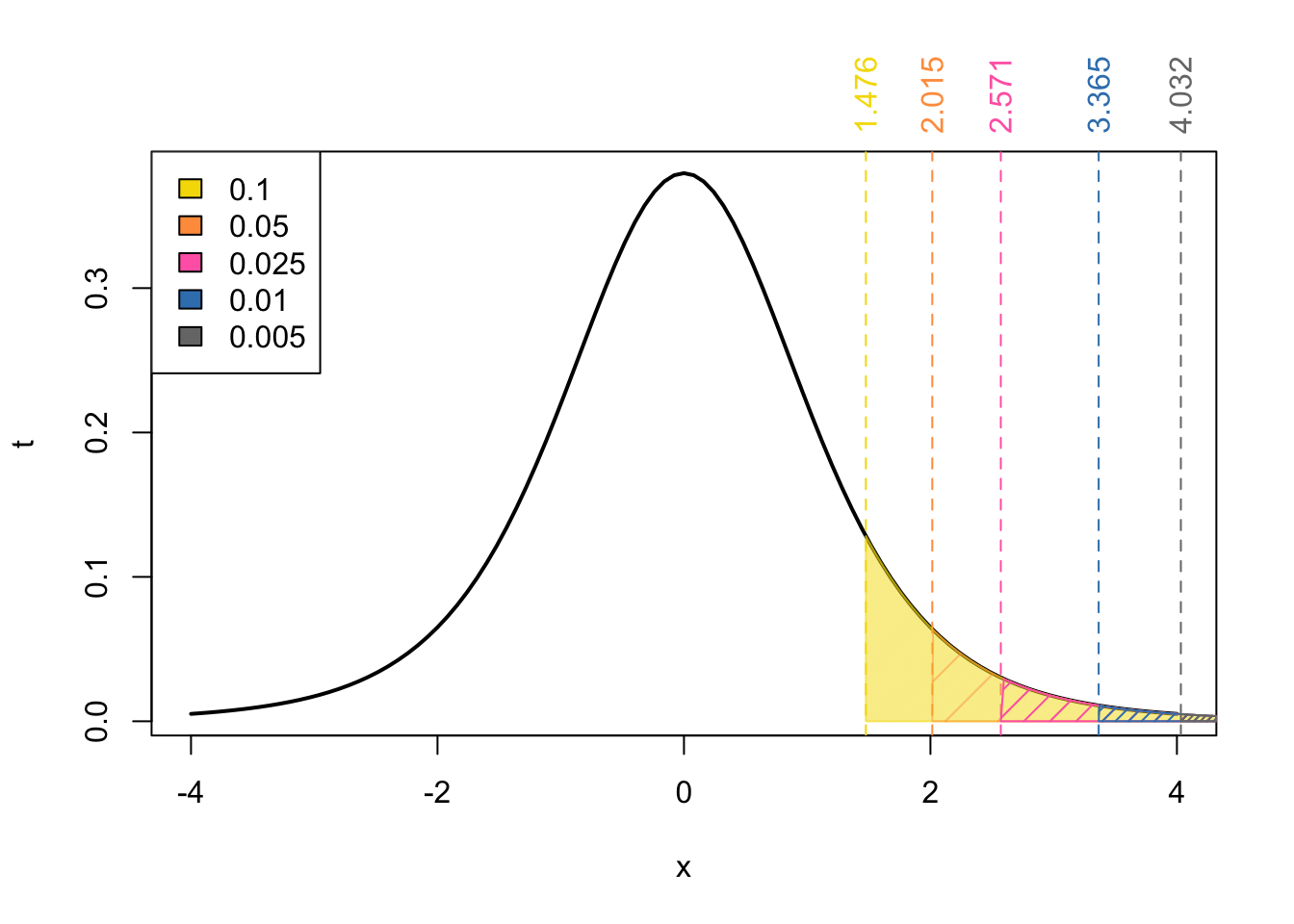
Next we find the neighbouring t-values for our \(t_{obs} = 2.75\):
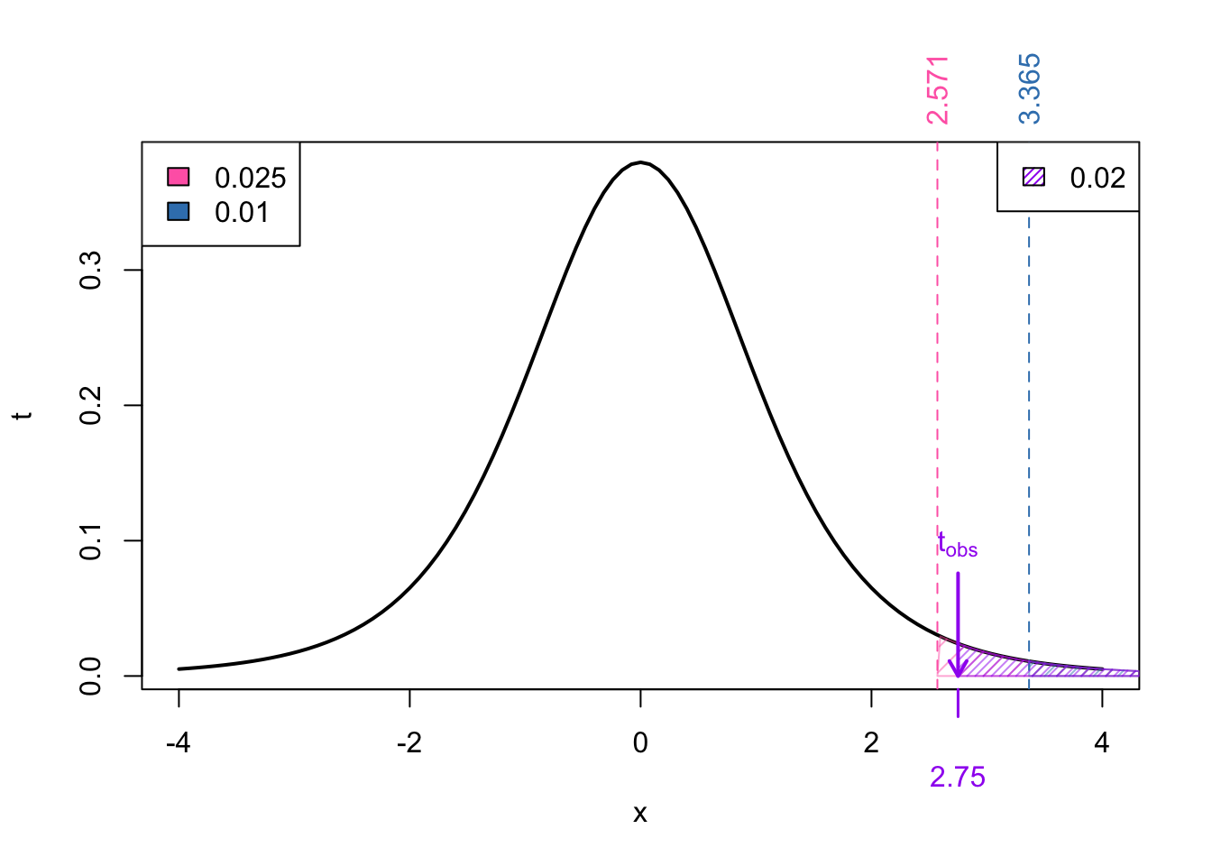
So now we can express the probability as:
\[ \begin{align} p-\text{value} &= \Pr(t_{\nu} > t_{obs}) = \Pr(t_{5} > 2.75) \end{align} \]
From Figure 4 we know that
\[\begin{align} \Pr(t_{5} > 3.365) < & \Pr(t_{5} > 2.75) < \Pr(t_{5} > 2.571) \\ \implies \text{area in blue} < & \ p-\text{value} < \text{area in pink}\\ 0.02 < & \ p-\text{value} < 0.05 \end{align}\]
We can find the exact p-value in R using:
pt(2.75, df = 5, lower.tail = FALSE)[1] 0.02015511Lower tail p-value
If we instead wanted the \(p\)-value associated with the lower tailed tests, from the symetric of the problem we would have:
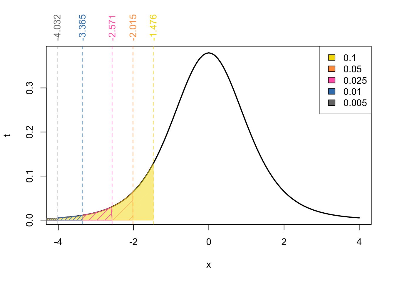
In this case, our observed test statistic \(t_{obs}\) only has a single neighbour:
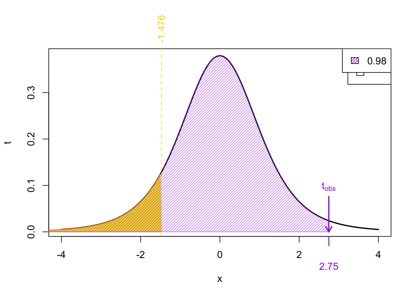
From Figure 5 we know that
\[\begin{align} \Pr(t_{5} < 2.75) &> \Pr(t_{5} < -1.476) \\ \implies \ p-\text{value} &> \text{area in yellow}\\ \ p-\text{value} &> 0.1 \end{align}\]
NOTE: Really, in this case we could say that \(p\)-value > 0.5 since we know3 that \(\Pr(t_{\nu} .< 0 ) = 0.5)\)
We can find the exact p-value in R using:
pt(2.75, df = 5)
pt(2.75, df = 5, lower.tail = TRUE) # same as above
[1] 0.9798449Two-sided p-value
For the two-tailed test, our reference values are
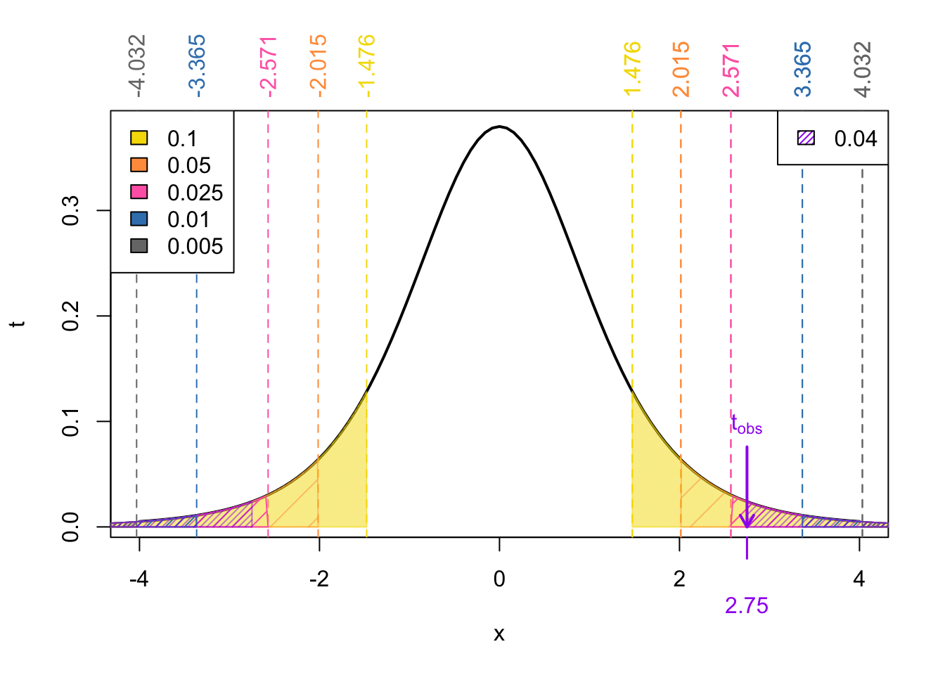
In this case, the neighbouring values of our test statistic \(t_{obs}\) is the same as the upper-tailed test:
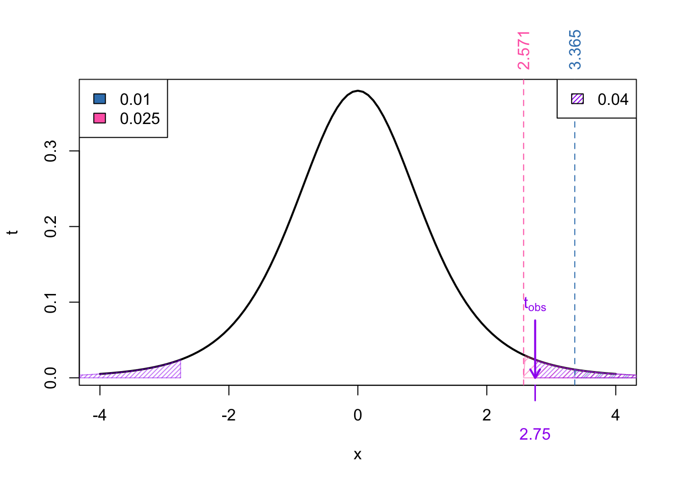
However, we we calculate the range for the \(p\)-value, we mustn’t forget to multiple by 2.
\[ \begin{align} p-\text{value} &= 2\times \Pr(t_{\nu} > | t_{obs}|) = 2\times\Pr(t_{5} > 2.75) \end{align} \]
From Figure 6 we know that
\[\begin{align} \Pr(t_{5} > 3.365) < & \Pr(t_{5} > 2.75) < \Pr(t_{5} > 2.571) \\ \implies 2\times\Pr(t_{5} > 3.365) < & \ 2\times\Pr(t_{5} > 2.75) < 2\times\Pr(t_{5} > 2.571) \\ \implies 2\times\text{area in pink} < & \ p-\text{value} < 2\times\text{area in blue} \\ 0.025 < & \ p-\text{value} < 0.05 \end{align}\]
We can find the exact p-value in R using:
2*pt(abs(2.75), df = 5, lower.tail = FALSE)[1] 0.04031022Two-sample Hypothesis Tests for the mean
Two-sample t-tests are hypothesis tests used to compare the means of two groups or populations. They determine whether there is a significant difference between the means of the two groups. There are three types that we discussed:
Paired t-test
In R:
## Paired t-test in R
t.test(x, y, paired = TRUE)
Pooled t-test
Checking for equal Variance
Before using the pooled t-test, it’s essential to check whether the variances of the two groups being compared are approximately equal. Here’s how you can check for equal variances:
- Visual Inspection: Plot the data using boxplots for each group. If the spread (i.e., the size of the boxes) looks similar between the groups, it suggests that the variances might be approximately equal.
- Rule of thumb: If the ratio of these the two sample standard deviations falls within 0.5 to 2, then it may be safe(ish) to assume equal variance.
If these checks are not met, proceed to Welch’s Procedure
In R:
## Pooled t-test in R
t.test(x, y, var.equal = TRUE)
Welch’s Procedure
In R:
## Paired t-test in R
t.test(x, y)
Two-sample Hypothesis Tests for proportions
We compare proportions from two independent groups (e.g., treatment vs control). Let:
\(p_1, p_2\): population proportions
\(\hat{p}_1 = \frac{x_1}{n_1}\), \(\hat{p}_2 = \frac{x_2}{n_2}\): sample proportions
Comparing Two Proportions
Used to test whether two population proportions are equal:
\[ H_0: p_1 = p_2 \quad \text{vs} \quad H_A: p_1 \ne p_2 \] or equivalently:
\[ H_0: p_1 - p_2 = 0 \quad \text{vs} \quad H_A: p_1 - p_2 \ne 0 \]Sample proportions:
\[ \hat{p}_1 = \frac{x_1}{n_1}, \quad \hat{p}_2 = \frac{x_2}{n_2} \]Pooled proportion (for hypothesis test):
\[ \hat{p} = \frac{x_1 + x_2}{n_1 + n_2} \]Test statistic:
\[ z = \frac{\hat{p}_1 - \hat{p}_2}{\sqrt{ \hat{p}(1 - \hat{p}) \left( \frac{1}{n_1} + \frac{1}{n_2} \right) }} \]Confidence interval (do not pool):
\[ SE = \sqrt{ \frac{\hat{p}_1(1 - \hat{p}_1)}{n_1} + \frac{\hat{p}_2(1 - \hat{p}_2)}{n_2} } \] \[ \text{CI: } (\hat{p}_1 - \hat{p}_2) \pm z^* \cdot SE \]Conditions:
- Independent random samples
- Success-failure condition: each group must have at least 10 successes and 10 failures
\[ n_1\hat{p}_1,\, n_1(1 - \hat{p}_1),\, n_2\hat{p}_2,\, n_2(1 - \hat{p}_2) \ge 10 \]
- Independent random samples
prop.test() in R
- Performs a hypothesis test for one or more proportions (based on a normal approximation).
- Can be used for:
- One proportion: test if a single proportion equals a hypothesized value.
- Two proportions: test if two population proportions are equal (no need to manually pool).
Syntax:
prop.test(x, n, p = NULL, alternative = "two.sided", conf.level = 0.95)x: number of successes (can be a vector for multiple groups)n: sample size(s)p: hypothesized proportionalternative:"two.sided","less", or"greater"
Automatically calculates and returns:
test statistic (which I won’t ask you to interpret for now)
\(p\)-value
confidence interval for the difference in proportions
Example:
Tests whether the proportions from two groups (30/100 vs. 45/120) are equal.
prop.test(c(30, 45), c(100, 120))
    2-sample test for equality of proportions with continuity correction

data:  c(30, 45) out of c(100, 120)
X-squared = 1.0521, df = 1, p-value = 0.305
alternative hypothesis: two.sided
95 percent confidence interval:
 -0.20894612  0.05894612
sample estimates:
prop 1 prop 2
 0.300  0.375
Note: without specifying a p, this test defaults to testing for a difference in proportions = 0.
Confidence Intervals
For each of the hypothesis tests above, we have a corresponding confidence interval. We will only concern ourselves with the “symmetric” confidence intervals in which \(\alpha\) is evenly split between the two tails. The generic form is:
\[ \begin{align} \text{point estimate} &\pm \underbrace{\text{critical value} \times SE}_{\text{Margin or Error}} \end{align} \]
Under the assumptions outlined in the corresponding hypothesis test section, the CI are given by:
CI for population mean (\(\sigma\) known)
A 100*(1- \(\alpha\))% confidence interval (CI) for \(\mu\) when the population variance \(\sigma^2\) is known is given by:
\[ \bar x \pm z^* \times \sigma/\sqrt{n} \]
where
- \(\bar x\) is the sample mean
- \(n\) is the sample size and
- \(z^*\) is the critical value that satisfies: \(\Pr(Z > z^*) = \alpha/2\)
Assumptions: When the sample data is a SRS (simple random sample) from the population of interest, this CI is exact when the population is normal, and approximate when \(n \geq 30\) (as a rough guideline).
CI for population mean (\(\sigma\) unknown)
A 100*(1- \(\alpha\))% confidence interval (CI) for \(\mu\) when the population variance \(\sigma^2\) is unknown is given by:
\[ \bar x \pm t^* \times s/\sqrt{n} \]
where
- \(\bar x\) is the sample mean
- \(n\) is the sample size and
- \(t^*\) is the critical value that satisfies: \(\Pr(t_\nu > t^*) = \alpha/2\)
Assumptions: When the sample data is a SRS (simple random sample) from the population of interest, this CI is exact when the population is normal, and approximate when \(n \geq 30\) (as a rough guideline).
CI for population proportion
A 100*(1- \(\alpha\))% confidence interval (CI) for the population proportion \(p\) is given by:
\[ \hat p \pm z^* \times \sqrt{\dfrac{\hat p (1 - \hat p)}{n}} \]
where
- \(\hat p\) is the sample proportion.
- \(n\) is the sample size and
- \(z^*\) is the critical value that satisfies: \(\Pr(Z > z^*) = \alpha/2\)
Assumptions: The sample is drawn from a binomial distribution and we satisfy the success-failure condition for normal approximation to be valid (we use and \(n\hat p \geq 10\) and \(n(1-\hat p) \geq 10\) .
Checking the normality assumption
If the sample size is large (typically above 30), the Central Limit Theorem suggests that the distribution of sample means will be approximately normal regardless of the distribution of the original data. In such cases, normality assumptions are often assumed to be met.
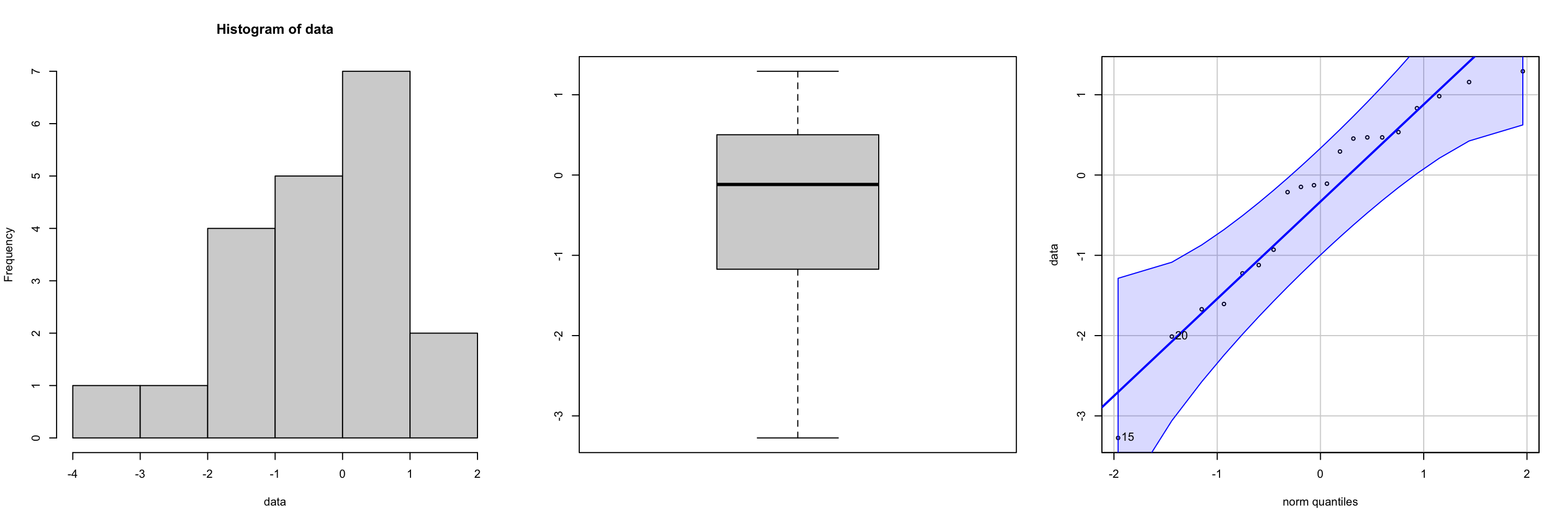
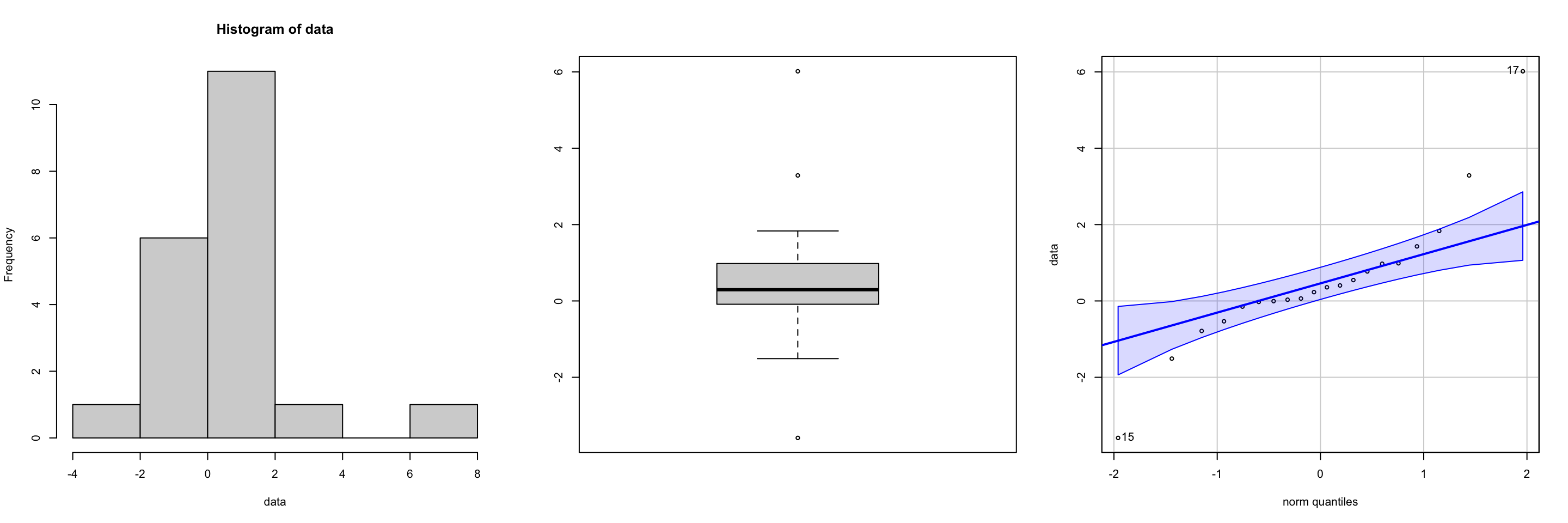
For small sample sizes you can use graphical methods, such as histograms, boxplots, or Q-Q plot to check the normality assumption for both one-sample z-test, t-tests, and chi-squared tests. See Figure 7 and Figure 8 for “good” and “bad” plots respectively.
To check the normality assumption using the Shapiro-Wilk test in R, you can use the shapiro.test() function.
Null hypothesis \(H_0\): The data comes from a normal distribution
Alternative hypothesis \(H_A\): The data does not come from a normal distribution
Have a numeric vector of data, say x:
x <- c(4.1, 3.8, 4.3, 4.0, 4.5, 3.9, 4.2)
shapiro.test(x)
    Shapiro-Wilk normality test

data:  x
W = 0.98384, p-value = 0.976
The test returns:
W statistic (not often interpreted directly)
\(p\)-value
Decision rule:
If \(p\)-value > \(\alpha\) : Fail to reject \(H_0\) → no evidence against normality ✅
If \(p\)-value \(\leq \alpha\): Reject \(H_0\) → evidence the data is not normal ❌
Connection between CI and two-sided tests
Two-sided hypothesis tests and confidence intervals (CI) are closely related statistical concepts that provide complementary information about a population parameter. The hypotheses for performing a two-sided test for a parameter \(\theta\) at a significance level of \(\alpha\) can be written: \[ \begin{align} &H_0: \theta = \theta_0 & &H_A: \theta \neq \theta_0 \end{align} \]
If we have a corresponding \(100*(1-\alpha\))% CI for \(\theta\), given by \([a, b]\) then a decision rule can be defined as follows:
If \(\theta_0\) is contained within \([a, b]\), we fail to reject the null hypothesis
If \(\theta_0\) is falls outside \([a, b]\), we reject the null hypothesis in favour of the two-sided alternative.
For one-sided tests, the logic is similar but the decision rule uses a one-sided confidence interval.
Left-tailed test
\[H_0: \theta = \theta_0 \quad \text{vs} \quad H_A: \theta < \theta_0\]
Use a 100(1 − \(\alpha\))% one-sided CI of the form:
\[(-\infty,\; b]\]
Decision rule:
If \(\theta_0 \leq b\): fail to reject \(H_0\)
If \(\theta_0 > b\) reject \(H_0\) in favor of the alternative
Right-tailed test
\[H_0: \theta = \theta_0 \quad \text{vs} \quad H_A: \theta > \theta_0\]
Use a 100(1 − \(\alpha\))% one-sided CI of the form:
\[[a, \infty)\]
Decision rule:
If \(\theta_0 \geq a\): fail to reject \(H_0\)
If \(\theta_0 < a\) reject \(H_0\) in favor of the alternative
Footnotes
This often involves assuming a specific distribution (e.g., normal distribution, t-distribution, chi-square distribution)↩︎
for demonstration sake, I will talk about the t-distribution but this will work for the Z-distributed test statistics as well.↩︎
remember: the area underneath the entire curve is 1. so the area under half of the curve must be 0.5.↩︎
