t.test(y ~ x, data = dataset)t-tests with formulas
STAT 205: Introduction to Mathematical Statistics
Introduction
The t.test() function in R is commonly used for hypothesis testing to compare the means of two groups. One way to use t.test() is by specifying a formula instead of providing separate vectors for the two groups. Formula notation simplifies the syntax and ensures that R correctly identifies the grouping variable.
Using Formulas in t.test()
The general syntax for t.test() using formula notation is:
where:
yis the numerical variable being tested (e.g., measurement values like reaction time or height).xis the categorical variable that defines the two groups. (i.e. a factor-type variable with two levels).datais the dataset containing both variables.
So your data might look something like this:
     y      x
1  x11 level1
2  x12 level1
3  x13 level1
4  x14 level1
5  x15 level1
6  x21 level2
7  x22 level2
8  x23 level2
9  x24 level2
10 x25 level2
where
\(x_{ij}\) is the \(j\)th observation from the \(i\)th group, and
level\(i\) corresponds to the \(i\) group.
How the Mean Difference is Formulated
When conducting a two-sample t-test using t.test(y ~ x), R automatically computes the difference as:
\[ \mu_{\text{level1}} - \mu_{\text{level2}} \]
where:
level1is the first level of the factor (reference level).level2is the second level of the factor.
To determine the reference level, use:
levels(dataset$group_variable)If the reference level does not correspond to your desired group, you can “relevel” (i.e. change the order of your categories) for the factor using:
dataset$group_variable <- relevel(dataset$group_variable, ref = "desired_reference_level")The sleep Dataset
The sleep dataset contains reaction time data for 10 individuals under two different conditions (groups 1 and 2). The dataset has three columns:
extra: The increase in hours of sleepgroup: The experimental group (factor with Drug 1 and Drug 2)ID: The individual subject identifier
data(sleep)
sleep
extra group ID
1 0.7 1 1
2 -1.6 1 2
3 -0.2 1 3
4 -1.2 1 4
5 -0.1 1 5
6 3.4 1 6
7 3.7 1 7
8 0.8 1 8
9 0.0 1 9
10 2.0 1 10
11 1.9 2 1
12 0.8 2 2
13 1.1 2 3
14 0.1 2 4
15 -0.1 2 5
16 4.4 2 6
17 5.5 2 7
18 1.6 2 8
19 4.6 2 9
20 3.4 2 10We would like to formally investigate if one drug better than the other at increasing the average hours of extra sleep.
Testing Assumptions
Visualizations
Stripchart
Code
stripchart(extra ~ group, data = sleep, pch = 16, col = c("skyblue", "firebrick"),
           vertical = TRUE, xlim = c(0.5, 2.5), xlab = "Soporific Drug No.",
           ylab = "Hours of Extra Sleep", main = "Effectiveness of Two Different Soporific Drugs \n at Increasing Sleep Times",
           method = "jitter", jitter = 0.1)  # <-- Jitter added

# Add reference line at 0
abline(h = 0, lty = 2, col = "gray")

# Compute means for each group
sleepmeans <- tapply(sleep$extra, sleep$group, mean)

# Add lines connecting the means
lines(sleepmeans ~ c(1,2), lty = 2, lwd = 2, col = "darkgray")

# Add points for group means
points(sleepmeans ~ c(1,2), pch = 3, cex = 2, col = c("skyblue", "firebrick"))

# Add a legend
legend("topleft", bty = "n", pch = 3, col = c("skyblue", "firebrick"),
       title = "Mean", legend = c("Drug 1", "Drug 2"))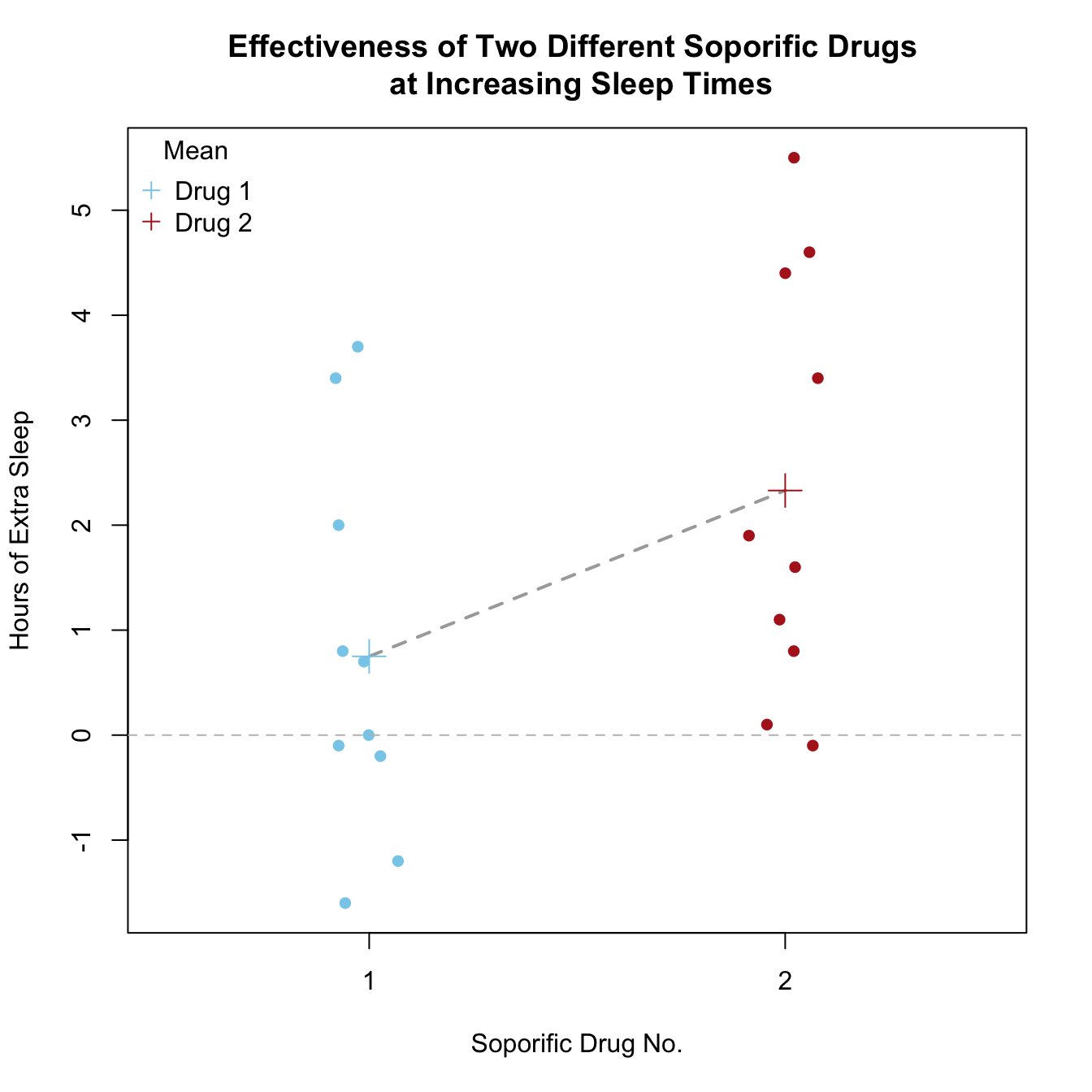
Overlapping Histograms
Code
# Overlapping histograms
hist(sleep$extra[sleep$group == "1"], col = rgb(0.4, 0.6, 0.8, 0.5),
     border = "black", breaks = 20, xlim = c(-2, 5), ylim = c(0, 6),
     xlab = "Hours of Extra Sleep", main = "Distribution of Extra Sleep by Drug",
     freq = TRUE)
hist(sleep$extra[sleep$group == "2"], col = rgb(0.8, 0.2, 0.2, 0.5),
     border = "black", breaks = 20, add = TRUE, freq = TRUE)

legend("topright", legend = c("Drug 1", "Drug 2"), fill = c(rgb(0.4, 0.6, 0.8, 0.5),
        rgb(0.8, 0.2, 0.2, 0.5)), border = "black", bty = "n")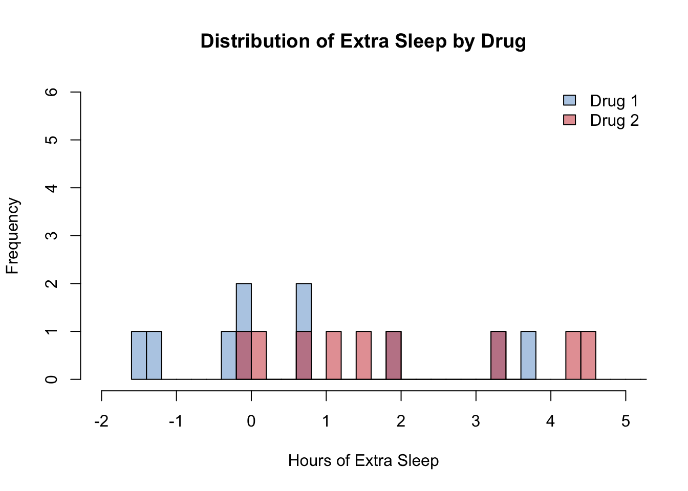
Side-by-side Boxplots
Code
# Side-by-side boxplot
boxplot(extra ~ group, data = sleep, col = c("skyblue", "firebrick"),
        xlab = "Soporific Drug No.", ylab = "Hours of Extra Sleep",
        main = "Comparison of Extra Sleep by Drug")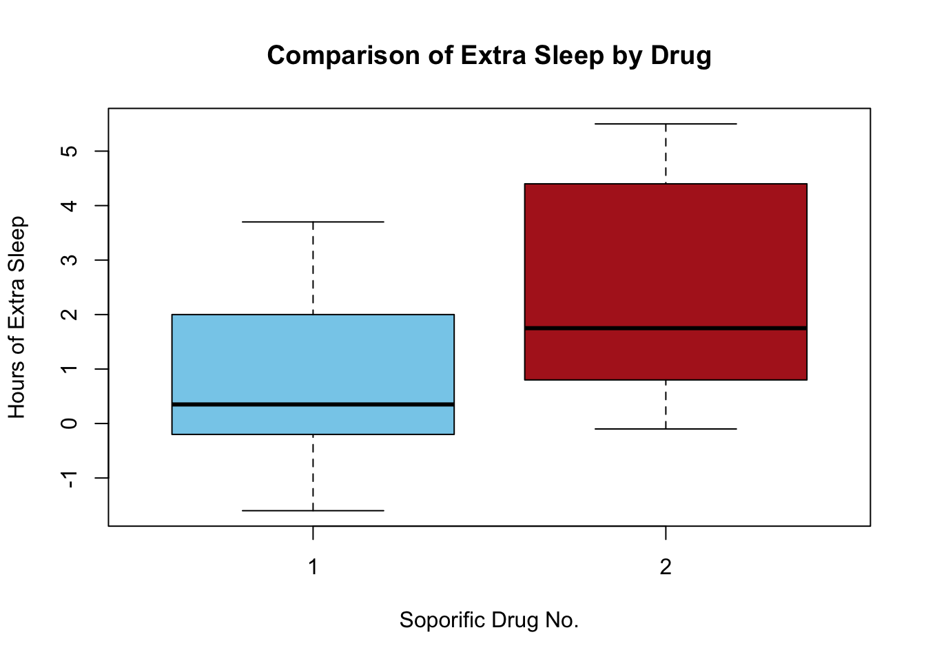
Side-by-Side Violin Plot (using ggplot2)
Code
library(ggplot2)

# Violin plot
ggplot(sleep, aes(x = group, y = extra, fill = group)) +
  geom_violin(alpha = 0.5, trim = FALSE) +
  geom_boxplot(width = 0.1, fill = "white") +  # Adds small boxplot inside
  scale_fill_manual(values = c("skyblue", "firebrick")) +
  labs(x = "Soporific Drug No.", y = "Hours of Extra Sleep",
       title = "Violin Plot of Extra Sleep by Drug") +
  theme_minimal()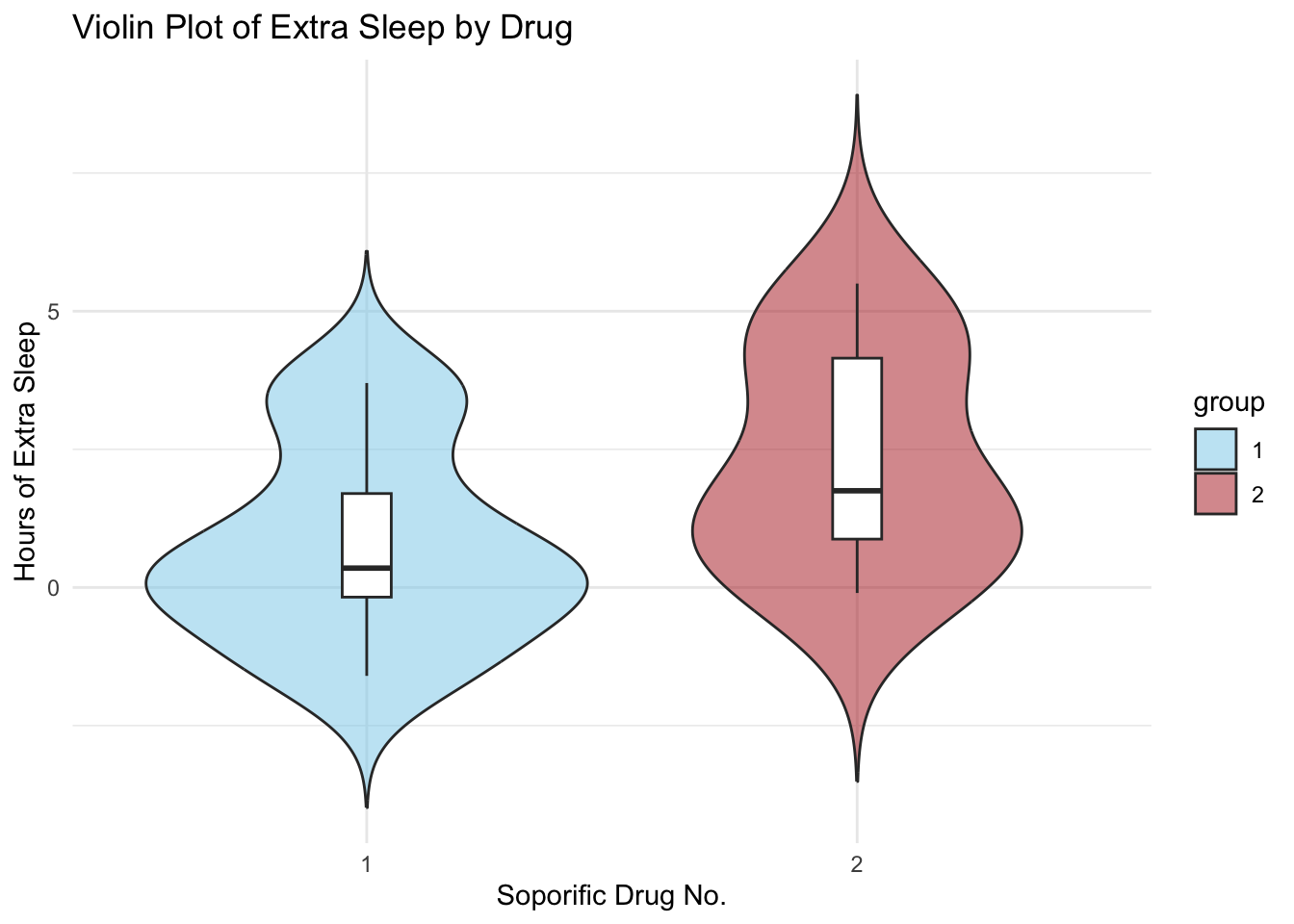
Paired \(t\)-test
Since these are the same individuals that we are taking measurements on, this is paired t-test.
The paired t-test does not support the formula method.
Hence the following will produce an error:
t.test(extra ~ group, data = sleep, paired = TRUE)
# Error in t.test.formula(extra ~ group, data = sleep, paired = TRUE) :
  # cannot use 'paired' in formula method
Instead we will need to create separate vectors for each group.
t.test(sleep$extra[sleep$group == 1], sleep$extra[sleep$group == 2], paired = TRUE)
    Paired t-test

data:  sleep$extra[sleep$group == 1] and sleep$extra[sleep$group == 2]
t = -4.0621, df = 9, p-value = 0.002833
alternative hypothesis: true mean difference is not equal to 0
95 percent confidence interval:
 -2.4598858 -0.7001142
sample estimates:
mean difference
          -1.58
Independent Test
Let’s pretend for the sake of demonstration, that these were independent individuals in this sample, i.e. the 10 people given Drug 1 were different than the 10 people given Drug 2. Then we would need to decide
if the equal variance assumption is appropriate (in which case we perform the pooled t-test)
if it is not safe to assume equal variance (in which case we’ll do the Welch procedure).
Checking for Equal Variance
Rule of thumb check for equal variance
Code
# Compute variances for each group
n1 <- length(sleep$extra[sleep$group == "1"])
n2 <- length(sleep$extra[sleep$group == "2"])

var_level1 <- var(sleep$extra[sleep$group == "1"])
var_level2 <- var(sleep$extra[sleep$group == "2"])
sd1 <- sqrt(var_level1)
sd2 <- sqrt(var_level2)
Since the sample sizes are equal (\(n_1 = 10\) and \(n_2 = 10\)) and since the computed ratio of standard deviations falls within the guideline range for assuming equal variances:
\[ \begin{align} 0.5 < &\frac{s_1}{s_2} < 2\\ 0.5 < &\frac{\sqrt{3.2006}}{\sqrt{4.009}} < 2\\ 0.5 < &\frac{{1.789}}{{2.0022}} < 2\\ 0.5 < & 0.894 < 2 \end{align} \]
we can justify using the pooled variance t-test (assuming similar sample sizes).
Testing for Normality
To check if the extra sleep values in the sleep dataset are approximately normally distributed, we can use the Shapiro-Wilk test, Q-Q plots, and histograms.
Shapiro-Wilk
shapiro.test(sleep$extra[sleep$group == "1"]) # Normality test for Drug 1
    Shapiro-Wilk normality test

data:  sleep$extra[sleep$group == "1"]
W = 0.92581, p-value = 0.4079
Since \(p > 0.05\), we fail to reject \(H_0\) → No strong evidence against normality.
shapiro.test(sleep$extra[sleep$group == "2"]) # Normality test for Drug 2
    Shapiro-Wilk normality test

data:  sleep$extra[sleep$group == "2"]
W = 0.9193, p-value = 0.3511
Since \(p > 0.05\), we fail to reject \(H_0\) → No strong evidence against normality.
QQ-plots
Here I will demo how to do Q-Q Plot with Confidence Bands. It requires the qqPlot() function from the cars package.
Code
library(car) # For qqPlot functionLoading required package: carDataCode
# Q-Q plot with confidence bands for both groups
par(mfrow = c(1, 2))  # Split into two panels

qqPlot(sleep$extra[sleep$group == "1"], main = "Q-Q Plot: Drug 1",
       id = FALSE, col = "skyblue")  # id=FALSE removes point labels

qqPlot(sleep$extra[sleep$group == "2"], main = "Q-Q Plot: Drug 2",
       id = FALSE, col = "firebrick")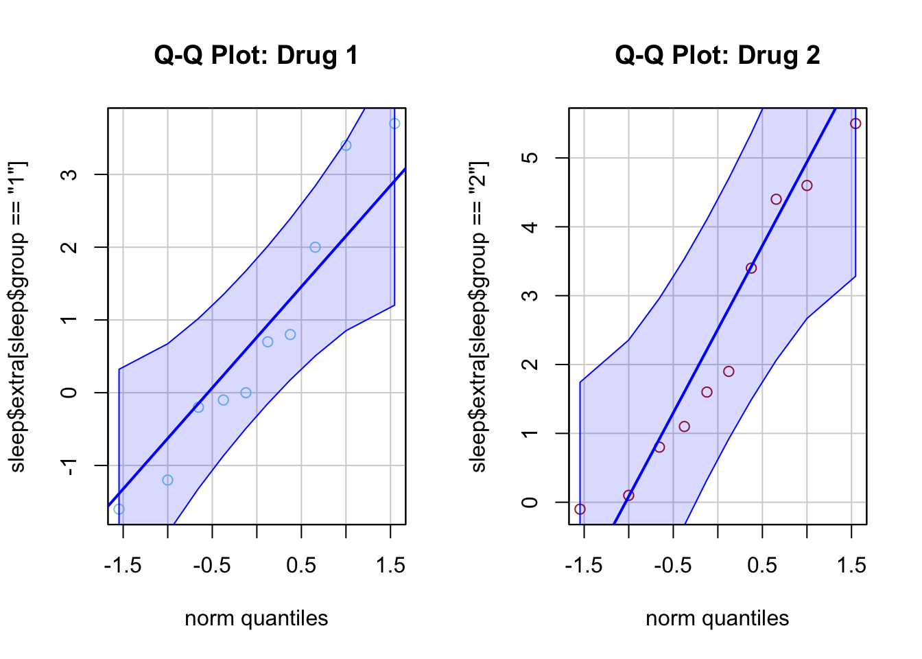
Code
par(mfrow = c(1, 1)) # Reset layoutWhy Use qqPlot() from car?
- It adds confidence bands (dashed lines) around the expected normal quantiles.
- If points stay within the bands, data is approximately normal.
- If points deviate significantly, normality might be questionable
Understanding the Q-Q Plot Components
- Points: Represent the actual data quantiles.
- Solid blue line: Represents the theoretical quantiles from a normal distribution.
- Shaded region (confidence band): Indicates the range within which we expect normal data to fall. Deviations outside this band suggest non-normality.
Drug 1 (Left Plot)
- Most points fall within the confidence band.
- A few minor deviations, but no extreme departures.
- Conclusion: Data appears reasonably normal for Drug 1.
Drug 2 (Right Plot)
- Most points stay within the confidence band.
- Some slight deviations, especially at the upper end.
- Conclusion: Data is approximately normal, though with slight skew or variability at higher values.
Overall Conclusion
Both groups do not show strong departures from normality. This supports the use of a t-test (assuming variance conditions are also met).
Independent Two-Sample t-Test
An independent two-sample t-test compares the means of two independent groups. In the sleep dataset, we compare extra sleep between group 1 and group 2.
Formula-Based Approach
Using formula notation, extra ~ group, R automatically determines the grouping variable and assumes the null hypothesis of:
\[ H_0: \mu_d = \texttt{mu0} \quad H_A: \mu_D\ \texttt{alternative} \ \texttt{mu0}\]
where \(\mu_d = \mu_{drug1} - \mu_{drug2}\). Recall
levels(sleep$group)[1] "1" "2"The computed test statistic will depend on what test we are doing (paired, pooled, or Welsh).
| Paired \(t\)-test | Pooled \(t\)-test | Welch |
|---|---|---|
t.test(x,y, paired=T) |
t.test(x,y, var.equal = T) |
t.test(x,y) |
| dependent groups | independent groups (\(\sigma_1 = \sigma_2\)) | independent groups (\(\sigma_1 \neq \sigma_2\)) |
| \((x_1, y_1), \dots, (x_n, y_n)\) \(d_i = x_i - y_i\) |
\((x_1, \dots, x_{n_1})\) , \((y_1, \dots, y_{n_2})\) | \((x_1, \dots, x_{n_1})\) , \((y_1, \dots, y_{n_2})\) |
| \[\dfrac{\overline{x}_{d} - \delta_0}{\dfrac{s_{d}}{\sqrt{n}}} \sim t_{n-1}\] | \[ \dfrac{\overline{x} - \overline{y} - \delta_0}{\sqrt{\dfrac{s_p^2}{{n_1}}+ \dfrac{s_p^2}{{n_2}}}} \sim t_{n1 + n2 -2} \] | \[ \dfrac{\overline{x} - \overline{y} - \delta_0}{\sqrt{\dfrac{s_1^2}{{n_1}}+ \dfrac{s_2^2}{{n_2}}}} \sim t_{\nu_w} \] |
In our case, we are adopting the equal variance assumption, so we will do the pooled test:
t.test(extra ~ group, data = sleep, var.equal = TRUE)
    Two Sample t-test

data:  extra by group
t = -1.8608, df = 18, p-value = 0.07919
alternative hypothesis: true difference in means between group 1 and group 2 is not equal to 0
95 percent confidence interval:
 -3.363874  0.203874
sample estimates:
mean in group 1 mean in group 2
0.75 2.33 After running t.test(), always check the “alternative hypothesis:” line in the output to confirm that R is testing the hypothesis you intended.
Welch Procedure
For the sake of completion, if we did not deem it safe to assume equal variance, we could perform the Welch procedure using:
t.test(extra ~ group, data = sleep)
    Welch Two Sample t-test

data:  extra by group
t = -1.8608, df = 17.776, p-value = 0.07939
alternative hypothesis: true difference in means between group 1 and group 2 is not equal to 0
95 percent confidence interval:
 -3.3654832  0.2054832
sample estimates:
mean in group 1 mean in group 2
           0.75            2.33