Post-Midterm Review

Author

Dr. Irene Vrbik

Exam Format

Coverage: All lectures and assignments (with heavier weight on the second have of the course)

Location: Please consult the exam scedule

Duration: 2.5 hours (150 minutes)

The exam will be a mix of

Multiple choice,
True/False (with supporting statements required),
Short Answer and
Long Answer

Material provided:

Standard normal table
Student $t$-distribution table
Chi-squared distribution table
Instructor formula sheet (work in progress!)

Other permitted material:

Non-graphing, non-programmable, calculator (e.g. Casio FX-991, Sharp EL-W516, EL-520 , Texas Instruments TI-36X Pro, CASIO fx-991ES PLUS C*). If you are unsure if your calculator is permitted, please ask me ASAP.
One standard page cheat sheet (front and back). You will be required to hand this in at the end of the test.

Post-midterm review

While there will be a heavier weight associated with the post-midterm topics, be sure to consult the midterm-review in addition to this document since the exam is cumulative!

A summary of the hypothesis tests we have covered.

Hypothesis Testing

Hypothesis testing is a statistical method used to make inferences about a population parameter based on sample data. It involves setting up two competing hypotheses, the null hypothesis ($H_0$) and the alternative hypothesis ($H_A$), and testing whether the evidence from the sample supports rejecting the null hypothesis in favor of the alternative hypothesis.

Here are the basic steps involved in hypothesis testing:

1. State the Hypotheses:

Null Hypothesis ($H_0$): Represents the default assumption, often stating that there is no effect or no difference (i.e. no-change or status-quo).
Alternative Hypothesis($H_A$): Represents the claim or research question you are testing for, stating that there is an effect or a difference.

2. Choose the Significance Level ($\alpha$)

This is the probability of rejecting the null hypothesis when it is actually true.
Common choices for $\alpha$ include 5% (most common) or 1%, 2%, or 10%

3. Select a Statistical Test

Choose an appropriate statistical test based on the type of data and the hypothesis being tested. Common tests include t-tests, z-tests, chi-square tests, ANOVA, etc.

4. Collect Data and Calculate Test Statistic

Collect a sample of data from the population of interest.
Calculate the appropriate test statistic based on the chosen test and the sample data.

5. Determine the Distribution of the Test Statistic

Under the null hypothesis, determine the distribution of the test statistic.
This often involves assuming a specific distribution (e.g., normal distribution, t-distribution, chi-square distribution).

6. Calculate Critical Value or p-value

Based on the assumed sampling distribution of the test statistic, calculate either the critical value or the $p$-value.

7. Make a Decision

For the critical value approach: if the test statistic falls with the rejection region, reject $H_0$ in favour of $H_A$, otherwise, fail to reject $H_0$.
For the $p$-value approach: if the $p$-value is less than the significance level ($\alpha$), reject $H_0$ in favour of $H_A$, otherwise, fail to reject $H_0$.

8. Draw Conclusions

Based on the decision in step 7, draw conclusions about the population parameter being tested.
Interpret the results in the context of the research question or problem being investigated.

Critical Value Approach

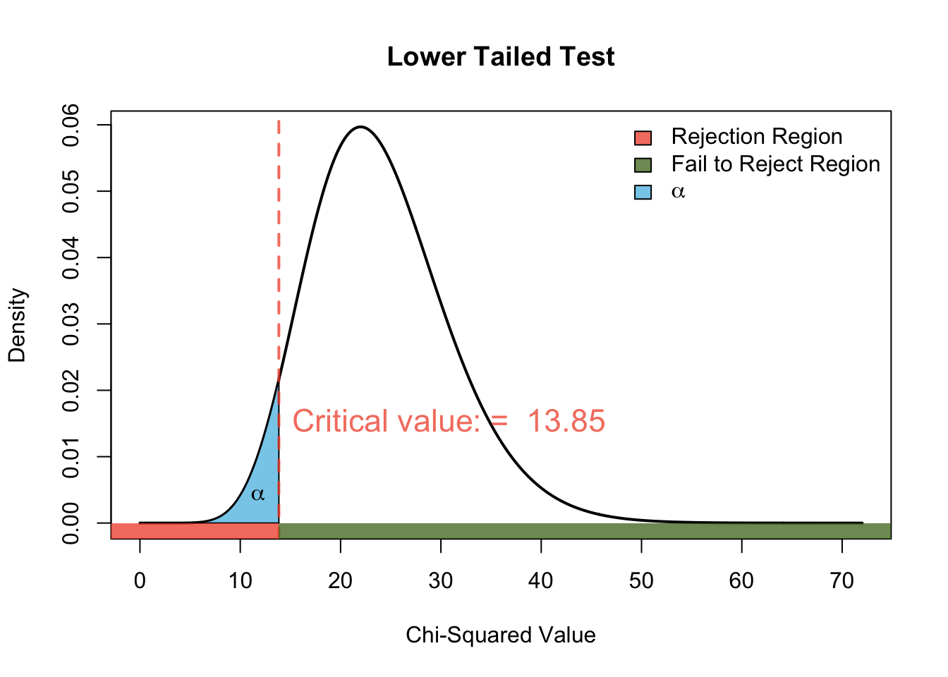
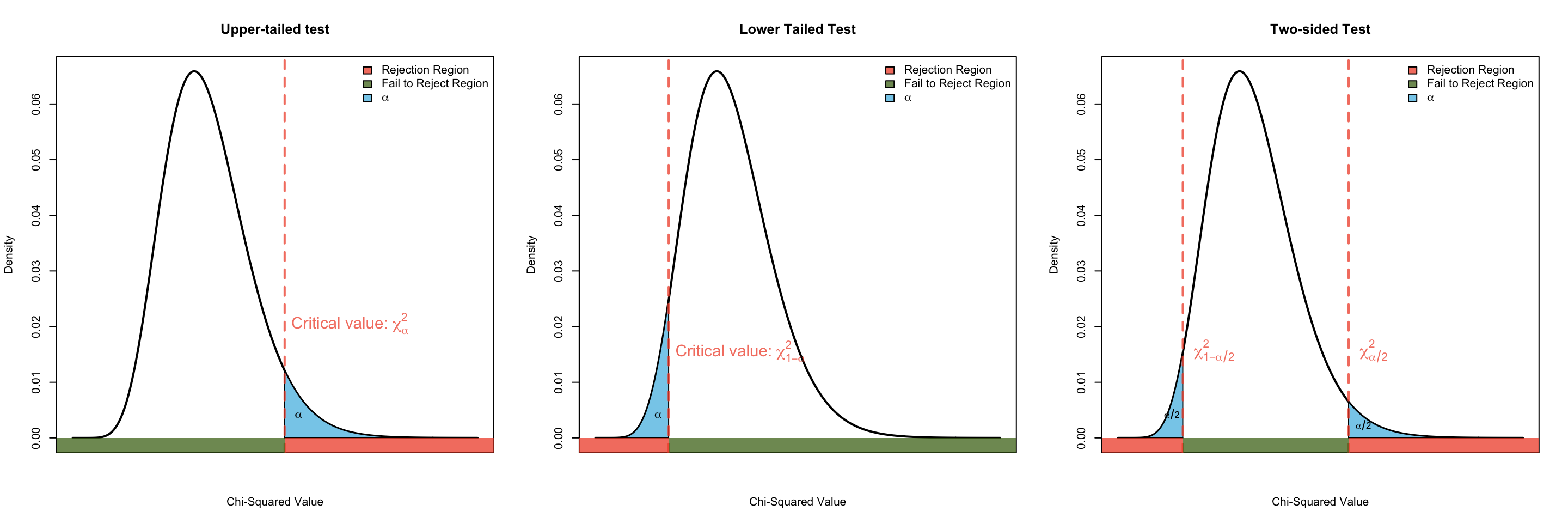
As it’s name suggests the critical value approach depends on the so-called critical value(s). These values define the so-called rejection region (as depicted in red in Figure 1) which comprise the set of values of the test statistic for which the null hypothesis is rejected. These boundaries are chosen based on:

the chosen significance level ($\alpha$),
the distribution of the test statistic under the null hypothesis, and
the specification of the alternative hypothesis $H_A$ (either two-tailed, lower-tailed, or upper-tailed).

If the observed test statistic falls within the rejection region, the $H_0$ is rejected in favour of $H_A$.

Critical Value approach

State hypotheses \[\begin{equation} H_0 : \theta = \theta_0 \quad \text{ vs } \quad H_A: \begin{cases} \theta \neq \theta_0& \text{ two-sided test} \\ \theta < \theta_0&\text{ one-sided (lower-tail) test} \\ \theta > \theta_0&\text{ one-sided (upper-tail) test} \end{cases} \end{equation}\]
Find critical value:

Figure 1: Visualization of the critical values and corresponding rejection regions for the three alternative hypotheses.
Compute the test statistic $\dfrac{\hat \theta- \theta_0}{SE(\hat \theta)}$
Conclusion: reject $H_0$ in favour of $H_A$ if observed test statistic falls within the rejection region, otherwise, fail to reject $H_0$.

P-value approach

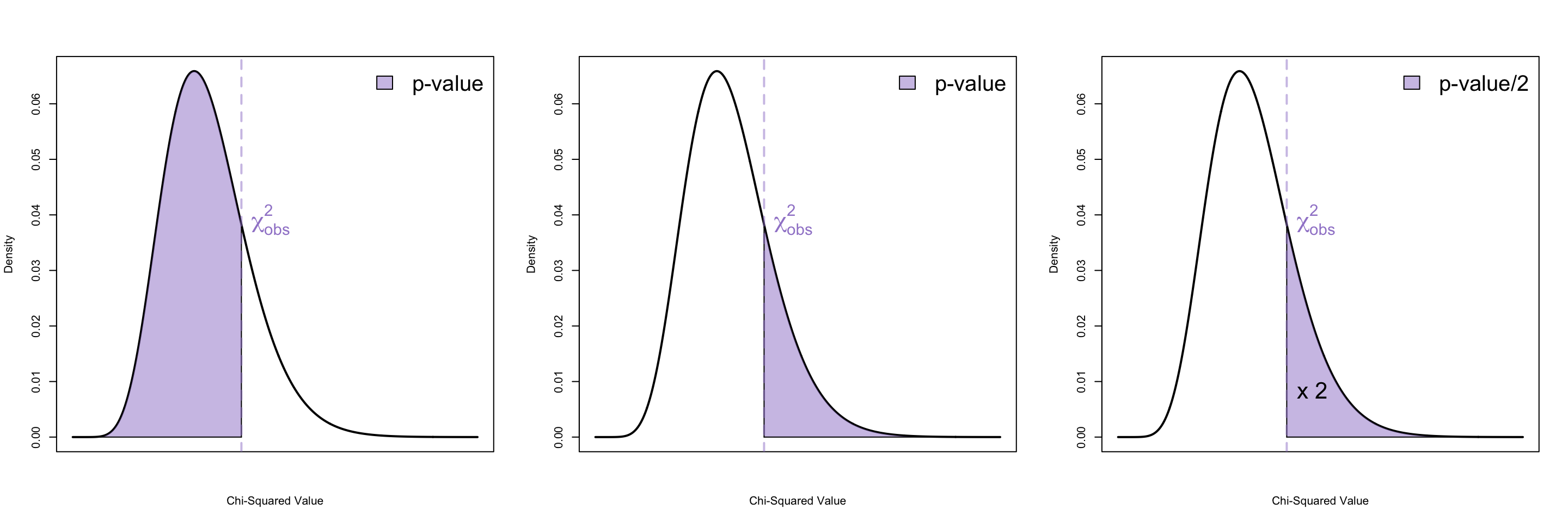
The $p$-value approach involves comparing a $p$-value with your significance level $\alpha$ (unless otherwise speicified, assumed to be 0.05). The $p$-value is the probability of observing a test statistic as extreme as, or more extreme (in the direction of $H_A$) than the one obtained from the sample data. If the $p$-value is less than $\alpha$, the null hypothesis is rejected in favour of the alternative hypothesis.

P-value approach

State hypotheses \[\begin{equation} H_0 : \theta = \theta_0 \quad \text{ vs } \quad H_A: \begin{cases} \theta \neq \theta_0& \text{ two-sided test} \\ \theta < \theta_0&\text{ one-sided (lower-tail) test} \\ \theta > \theta_0&\text{ one-sided (upper-tail) test} \end{cases} \end{equation}\]
Find critical value:
\[\begin{cases} P(-z_{crit} < Z < z_{crit}) = 1 - \alpha &\text{ if } H_A: \theta \neq \theta_0 \\ P(Z < z_{crit}) = \alpha &\text{ if } H_A: \theta < \theta_0 \\ P(Z > z_{crit}) = \alpha &\text{ if } H_A: \theta > \theta_0 \end{cases}\]
Compute the test statistic
Compute the $p$-value on the null distribution.

Visualization of the $p$-values and for the three alternative hypotheses.
Conclusion: reject $H_0$ if $p$-value is less than $\alpha$ otherwise, fail to reject $H_0$.

One-sample Hypothesis Tests

One-sample hypothesis tests are statistical tests used to make inferences about a population based on a single sample of data. These tests are commonly used when you have a sample of data and want to determine whether it’s reasonable to infer that the sample comes from a population with a specific characteristic or parameter. In this course we concern ourselves with tests for the population mean ($\mu$), population proportion ($p$), and population variance $\sigma^2$.

Z-tests

So called “z-test” are hypothesis tests in which the test statistic follows a standard normal distribution. The two tests we covered that fall into this category are:

Hypothesis test for the mean $\mu$ (with $\sigma$ known)
Hypothesis tests for the proportion $p$

Hypothesis test for the mean

Assumptions for the one-sample z-test

We have a simple random sample
The population from which the sample is drawn follows a normal distribution, or the sample size is large enough for the Central Limit Theorem to apply.
The population variance $\sigma^2$ is known.

Critical Value approach for a single population mean

State hypotheses \[\begin{equation} H_0 : \mu = \mu_0 \quad \text{ vs } \quad H_A: \begin{cases} \mu \neq \mu_0& \text{ two-sided test} \\ \mu < \mu_0&\text{ one-sided (lower-tail) test} \\ \mu > \mu_0&\text{ one-sided (upper-tail) test} \end{cases} \end{equation}\]
Find critical value:
\[\begin{cases} P(-z_{crit} < Z < z_{crit}) = 1 - \alpha &\text{ if } H_A: \mu \neq \mu_0 \\ P(Z < z_{crit}) = \alpha &\text{ if } H_A: \mu < \mu_0 \\ P(Z > z_{crit}) = \alpha &\text{ if } H_A: \mu > \mu_0 \end{cases}\]
Compute the test statistic $z_{obs} = \dfrac{\bar x - \mu_0}{\sigma/\sqrt{n}}.$
Conclusion: reject $H_0$ if $z_{obs} \in$ rejection region, otherwise, fail to reject $H_0$.

P-value approach for a single population mean

State hypotheses \[\begin{equation} H_0 : \mu = \mu_0 \quad \text{ vs } \quad H_A: \begin{cases} \mu \neq \mu_0& \text{ two-sided test} \\ \mu < \mu_0&\text{ one-sided (lower-tail) test} \\ \mu > \mu_0&\text{ one-sided (upper-tail) test} \end{cases} \end{equation}\]
Compute the test statistic $z_{obs} = \dfrac{\bar x - \theta_0}{\sigma/\sqrt{n}}.$
Compute the $p$-value on the null distribution.
Conclusion: reject $H_0$ if $p$-value is less than $\alpha$ otherwise, fail to reject $H_0$.

Hypothesis Tests for Proportions

Assumptions for Hypothesis Tests for Proportions

We have a simple random sample
The experiment can be modeled by the binomial distribution:
- number of trials is fixed
- trials are independent
- only two possible outcomes (‘success’ and ‘failure’)
- Probabilities constant for each trial
Success-failure condition¹: $np \geq 10$ and $n(1-p) \geq 10)$

Critical Value approach for proportions

State hypotheses \[\begin{equation} H_0 : p = p_0 \quad \text{ vs. } \quad H_A: \begin{cases} p \neq p_0& \text{ two-sided test} \\ p < p_0&\text{ one-sided (lower-tail) test} \\ p > p_0&\text{ one-sided (upper-tail) test} \end{cases} \end{equation}\]
Find critical value:
\[\begin{cases} P(-z_{crit} < Z < z_{crit}) = 1 - \alpha &\text{ if } H_A: p \neq p_0 \\ P(Z < z_{crit}) = \alpha &\text{ if } H_A: p < p_0 \\ P(Z > z_{crit}) = \alpha &\text{ if } H_A: p > p_0 \end{cases}\]
Compute the test statistic $z_{obs} = \dfrac{\hat p - p_0}{\sqrt{p_0(1-p_0)/n}}.$
Conclusion: reject $H_0$ if $z_{obs} \in$ rejection region, otherwise, fail to reject $H_0$.

$p$-value approach

State hypotheses \[\begin{equation} H_0 : p = p_0 \quad \text{ vs. } \quad H_A: \begin{cases} p \neq p_0& \text{ two-sided test} \\ p < p_0&\text{ one-sided (lower-tail) test} \\ p > p_0&\text{ one-sided (upper-tail) test} \end{cases} \end{equation}\]
Compute the test statistic $z_{obs} = \dfrac{\hat p - p_0}{\sqrt{p_0(1-p_0)/n}}.$
Calculate the $p$-value
\[\begin{cases} 2P(Z \geq |z_{obs}|) &\text{ if } H_A: p \neq p_0 \\ P(Z \leq z_{obs}) &\text{ if } H_A: p < p_0 \\ P(Z \geq z_{obs}) &\text{ if } H_A: p > p_0 \end{cases}\]
Conclusion: reject $H_0$ if $p$-value is less than $\alpha$ (typically 0.05), otherwise, fail to reject $H_0$.

t-test

A one-sample t-test is a statistical test used to determine whether the mean of a single sample differs significantly from a specified value. The one-sample t-test is typically used when the sample size is small (typically less than 30) or when the population standard deviation is unknown, while the one-sample z-test is used when the population standard deviation is known and the sample size is large (typically greater than 30).

Assumptions for the one-sample t-test

We have a simple random sample
The population from which the sample is drawn follows a normal distribution, or the sample size is large enough for the Central Limit Theorem to apply.

The test statistic for this test is

\[\dfrac{\bar x - \mu_0}{s/\sqrt{n}} \sim t_{\nu = n - 1}\] where

$s$ is the sample standard deviation
$\bar x$ is the sample mean
$n$ is the sample size
$\mu_0$ is the hypothesized value of population mean (aka null value)
$t_\nu$ represents the student-$t$ distribution with $\nu$ degrees of freedom

We then use the Critical Value Approach or P-value approach to make a decision.

Chi-squared test for variance

A chi-squared test for variance is a statistical method used to determine whether the variance of a dataset significantly differs from a specified variance, based on the chi-squared distribution.

The hypotheses we use is

\[ \begin{align} H_0: & \sigma^2 = \sigma_0^2 & H_A: & \begin{cases} \sigma^2 \neq \sigma_0^2\\ \sigma^2 < \sigma_0^2\\ \sigma^2 > \sigma_0^2 \end{cases} \end{align} \]

The test statistic we use for this test is:

\[ \dfrac{(n-1)s^2}{\sigma_0^2} \sim \chi^2_{\nu = n-1} \] where

$s^2$ is our sample variance
$n$ is our sample size
$\sigma_0^2$ is the hypothesized value of population variance, and
$\chi^2_{\nu}$ represents a chi-sqare distribution with $\nu$ degress of freedom.

Assumptions for the chi-square test for one-sample variance

A simple random sample from the population
A normally distributed population (very important, even for large sample sizes)

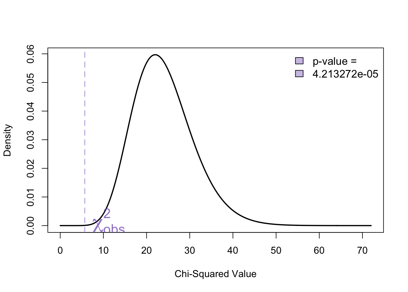
We then use the Critical Value Approach or P-value approach to make a decision.

The rejection region associated with an upper-tailed test (left), lower-tailed test (center) and two-sided test (right) for the population variance. Note that the critical value will depend on the chosen significance level ($\alpha$) and the d.f.

Similarly we can find $p$-values from Chi-squared tables or R

The $p$-values associated with an upper-tailed test (left), lower-tailed test (center) and two-sided test (right) for the population variance. Note that the critical value will depend on the chosen significance level ($\alpha$) and the d.f.

Exercise 1:

With individual lines at its various windows, a post office finds that the standard deviation for normally distributed waiting times for customers on Friday afternoon is 7.2 minutes. The post office experiments with a single, main waiting line and finds that for a random sample of 25 customers, the waiting times for customers have a standard deviation of 3.5 minutes.

With a significance level of 5%, test the claim that a single line causes lower variation among waiting times for customers.

Solution (click to view)

We can set up the test using the population variance as follows.

\[ \begin{align} H_0: & \sigma^2 = 7.2^2 & H_A: & \sigma^2 < 7.2^2 \end{align} \]

Test statistic

\[ \begin{align} \frac{(n-1)s^2}{\sigma_0^2} &\sim \chi^2_{\nu = n - 1 = 24} \\ \frac{(25-1)3.5^2}{7.2^2} &= 5.6712963 \end{align} \]

i) Either compare with critical value:

ii) or find the $p$-value

Relevant R code:

# Set the significance level (alpha)
alpha <- 0.05  # Change as needed

# Determine the degrees of freedom (df)
df <- 24  # Change as needed, typically df = n - 1

# Calculate the critical value from the chi-squared distribution
critical_valueL <- qchisq(alpha, df)
critical_valueL

[1] 13.84843

# Calculate the p-value from the chi-squared distribution
chi_obs = ((25-1)*3.5^2)/(7.2^2)
pval = pchisq(chi_obs, df = df)
pval

[1] 4.213272e-05

Decision: Since i) the observed test statistic falls in the rejection region or ii) the $p$-value is less that $\alpha = 0.05$, we reject the null hypothesis in favour of the alternative.

Conclusion: There is strong evidence to suggest that a single line results in lower variation among waiting times for customers.

Checking the normality assumption

If the sample size is large (typically above 30), the Central Limit Theorem suggests that the distribution of sample means will be approximately normal regardless of the distribution of the original data. In such cases, normality assumptions are often assumed to be met.

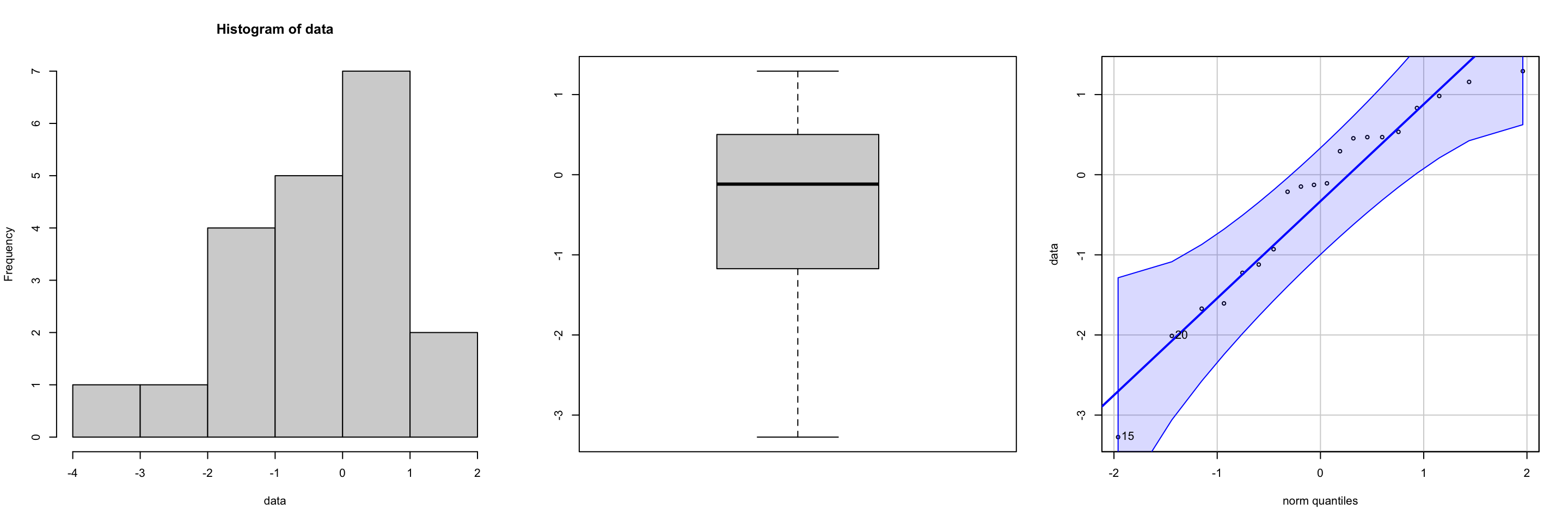
For small sample sizes you can use graphical methods, such as histograms, boxplots, or Q-Q plot to check the normality assumption for both one-sample z-test, t-tests, and chi-squared tests. See Figure 2 and Figure 3 for “good” and “bad” plots respectively.

Figure 2: Examples of of these plots from 20 randomly sampled observations from a normal distribution.

Figure 3: Examples of of these plots from 20 randomly sampled observations from a student-t distribution with 3 degrees of freedom.

Confidence Intervals

For each of the hypothesis tests above, we have a corresponding confidence interval. We will only concern ourselves with the “symmetric” confidence intervals in which $\alpha$ is evenly split between the two tails. The generic form is:

\[ \begin{align} \text{point estimate} &\pm \underbrace{\text{critical value} \times SE}_{\text{Margin or Error}} \end{align} \]

Under the assumptions outlined in the corresponding hypothesis test section, the CI are given by:

CI for population mean with know population variance

A 100*(1- $\alpha$)% confidence interval (CI) for $\mu$ when the population variance $\sigma^2$ is known is given by:

\[ \bar x \pm z^* \times \sigma/\sqrt{n} \]

where

$\bar x$ is the sample mean
$n$ is the sample size and
$z^*$ is the critical value that satisfies: $\Pr(Z > z^*) = \alpha/2$

CI for population mean with unknown population variance

A 100*(1- $\alpha$)% confidence interval (CI) for $\mu$ when the population variance $\sigma^2$ is unknown is given by:

\[ \bar x \pm t^* \times s/\sqrt{n} \]

where

$\bar x$ is the sample mean
$n$ is the sample size and
$t*$ is the critical value that satisfies: $\Pr(t_{n-1} > t^*) = \alpha/2$

CI for population proportion

A 100*(1- $\alpha$)% confidence interval (CI) for the population proportion $p$ is given by:

\[ \hat p \pm z^* \times \dfrac{\hat p (1 - \hat p)}{n} \]

where

$\hat p$ is the sample proportion.
$n$ is the sample size and
$z^*$ is the critical value that satisfies: $\Pr(Z > z^*) = \alpha/2$

CI for population variance

A 100*(1- $\alpha$)% confidence interval (CI) for the population variance $\sigma^2$ is given by:

\[ \left( \frac{(n-1)s^2}{\chi^2_{\alpha/2, n-1}}, \frac{(n-1)s^2}{\chi^2_{1-\alpha/2, n-1}} \right) \]

where

$s$ is the sample variance
$n$ is the sample size and
$\chi^2_L = \chi^2_{\alpha/2, n-1}$ and $\chi^2_U = \chi^2_{1-\alpha/2, n-1}$ are the critical values that respectively satisfy: \[ \begin{align} \Pr(\chi^2_{n-1} < \chi^2_L) &= \alpha/2\\ \Pr(\chi^2_{n-1} > \chi^2_U) &= \alpha/2 \end{align} \] where $\chi^2_{n-1}$ is a chi-square random variable with $\nu = n-1$ degrees of freedom.

Connection between CI and two-sided tests

Two-sided hypothesis tests and confidence intervals (CI) are closely related statistical concepts that provide complementary information about a population parameter. The hypotheses for performing a two-sided test for a parameter $\theta$ at a significance level of $\alpha$ can be written: \[ \begin{align} &H_0: \theta = \theta_0 & &H_A: \theta \neq \theta_0 \end{align} \]

If we have a corresponding $100*(1-\alpha$)% CI for $\theta$, given by $[a, b]$ then a decision rule can be defined as follows:

If $\theta_0$ is contained within $[a, b]$, we fail to reject the null hypothesis
If $\theta_0$ is falls outside $[a, b]$, we reject the null hypothesis in favour of the two-sided alternative.

Two-sample Hypothesis Tests for the mean

Two-sample t-tests are hypothesis tests used to compare the means of two groups or populations. They determine whether there is a significant difference between the means of the two groups. There are three types that we discussed:

Paired t-test
Pooled t-test
Welch’s Procedure

Paired t-test

Assumptions for the Paired t-test

Dependent observations: The observations within each pair are dependent, meaning they are not independent of each other.
Normally distributed differences: The differences between paired observations should follow a normal distribution.
Random sampling: The paired observations should be simple random sample from the population.

Paird t-test for the Difference of means for Dependent Groups

State hypotheses
\[\begin{align} H_0&: \mu_1 - \mu_2 = \delta_0 & H_A: \begin{cases} \mu_1 - \mu_2 \neq \delta_0 \\ \mu_1 - \mu_2 < \delta_0 \\ \mu_1 - \mu_2 > \delta_0 \end{cases} \end{align}\]
Test Statistic: $\quad \quad T = \dfrac {\bar{X}_1 - \bar{X}_2 - \delta} { s_d /\sqrt{ n }} \sim t_{\nu}$ where $\nu = n - 1$

where $s_d$ is the standard deviation of the paired differences $d_1, d_2, \dots, d_n$ and $d_i = x_{1i} - x_{2i}$ and $n$ is the number of matched pairs $(x_{11}, x_{21})$, $(x_{12}, x_{2})$, $\dots$, $(x_{1n}, x_{2n})$
Make a decision based on the Critical Value Approach or P-value approach
Conclusion: interpret the results of the test in the context of the research question or problem being investigated.

In R:

## Paired t-test in R
t.test(x, y, paired = TRUE)

Pooled t-test

Assumptions for the Pooled t-test

Equal variances: The populations from which the samples are drawn should have equal variances
Normality: The populations from which the samples are drawn should be approximately normally distributed.
Independent observations: The observations in each sample are independent of each other.
Random sampling: The samples should be randomly selected from their respective populations.

Checking for equal Variance

Before using the pooled t-test, it’s essential to check whether the variances of the two groups being compared are approximately equal. Here’s how you can check for equal variances:

Visual Inspection: Plot the data using boxplots for each group. If the spread (i.e., the size of the boxes) looks similar between the groups, it suggests that the variances might be approximately equal.
Rule of thumb: If the ratio of these the two sample standard deviations falls within 0.5 to 2, then it may be safe(ish) to assume equal variance.

If these checks are not met, proceed to Welch’s Procedure

Pooled t-test for the Difference of means for Independent Groups ($\sigma_1^2 = \sigma_2^2$)

State hypotheses
\[\begin{align} H_0&: \mu_1 - \mu_2 = \delta_0 & H_A: \begin{cases} \mu_1 - \mu_2 \neq \delta_0 \\ \mu_1 - \mu_2 < \delta_0 \\ \mu_1 - \mu_2 > \delta_0 \end{cases} \end{align}\]
Test Statistic: $\quad \quad T = \dfrac {\bar{X}_1 - \bar{X}_2 - \delta} { s_p \sqrt{ \dfrac{1}{n_1} + \dfrac{1}{n_2} }} \sim t_{\nu}$ where $\nu = n_1 + n_2 - 2$

where $s_p$ is the square-root of the pooled variance:

\[s_p^2 = \dfrac{(n_1 - 1)s_1^2 + (n_2 - 1)s_2^2}{n_1 + n_2 -2}\]

Make a decision based on the Critical Value Approach or P-value approach
Conclusion: interpret the results of the test in the context of the research question or problem being investigated.

In R:

## Pooled t-test in R
t.test(x, y, var.equal = TRUE)

Welch’s Procedure

Assumptions for the Welch Procedure

Normality: The populations from which the samples are drawn should be approximately normally distributed.
Independent observations: The observations in each sample are independent of each other.
Random sampling: The samples should be randomly selected from their respective populations.

Welch Procedure for the Difference of means for Independent Groups ($\sigma_1^2 \neq \sigma_2^2$)

State hypotheses
\[\begin{align} H_0&: \mu_1 - \mu_2 = \delta_0 & H_A: \begin{cases} \mu_1 - \mu_2 \neq \delta_0 \\ \mu_1 - \mu_2 < \delta_0 \\ \mu_1 - \mu_2 > \delta_0 \end{cases} \end{align}\]
Test Statistic: $\quad \quad T = \dfrac {\bar{X}_1 - \bar{X}_2 - \delta} {\sqrt{ \dfrac{S_1^2}{n_1} + \dfrac{S_2^2}{n_2} }} \sim t_{\nu}$ where $\nu = \frac{\left( \frac{s_1^2}{n_1} + \frac{s_2^2}{n_2} \right)^2}{\frac{1}{n_1 - 1}\left( \frac{s_1^2}{n_1} \right)^2 + \frac{1}{n_2 - 1} \left( \frac{s_2^2}{n_2} \right)^2}$

and $s_1^2$ and $s_2^2$ are the sample variances calculated using: \[\begin{align} s_1^2 &= \dfrac{\sum_{i = 1}^{n_1} (x_{1i} -\bar x_{1} )^2 }{n_1 - 1} & s_2^2 &= \dfrac{\sum_{i = 1}^{n_2} (x_{2i} -\bar x_{2} )^2 }{n_2 - 1} \end{align}\]

Make a decision based on the Critical Value Approach or P-value approach
Conclusion: interpret the results of the test in the context of the research question or problem being investigated.

In R:

## Paired t-test in R
t.test(x, y)

ANOVA

Analysis of Variance (ANOVA) is a statistical method used to compare the means of three or more groups to determine if at least one group mean is significantly different from the others. In other words:

\[ \begin{align} &H_0: \mu_1 = \mu_2 = \dots = \mu_k \quad \text{ or } \quad \ H_0: \text{ all group means are equal}\\ &H_A: \text{At least one } \mu_i \text{ is different from the others.} \end{align} \]

Assumptions for using ANOVA

Random sampling: The observations are independent simple random samples from the populations
Normality: The populations are normally distributed
Equal variance: The population variances are equal

Non-extreme departures from the normality assumes are not that serious since the sampling distribution of the test statistic is fairly robust, especially as sample size increases sample sizes for all groups are equal. Akin to the rule of thumb checks used for the pooled $t$-test, we could compare the smallest and largest sample standard deviations. If the ratio of these two sample standard deviations falls within 0.5 to 2, we will deem it reasonable to assume equal variance.

The calculations for this test are done using software like R and typically stored in an ANOVA table with the following structure …

ANOVA table

Source	df	SS	MS	F	$p$-value
Between	$k - 1$	SSB	MSB	$\frac{MSB}{MSW}$	$\Pr(F_{df_B, df_W} > F_{obs})$
Within	$n- k$	SSW	MSW
Total	$n-1$	TSS

$df_T = df_B + df_W = n - 1$
- $df_B= k - 1$
- $df_W = n-k$
$TSS = SSW + SSB$
$MSB = SSB/df_B$
$MSW = SSW/df_W$

The test statistic used is:

\[ \dfrac{MSB}{MSW} = \dfrac{SSB/df_b}{SSW/df_w} \sim F_{df_B, df_W} \]

where $F_{\nu_1, \nu_2}$ denotes the $F$ distribution with numerator degrees of freedom given by $\nu_1$ and denominator degrees of freedom given by $\nu_2$.

While the critical value could be used in these scenarioes, we will exclusively be making our decision based on the $p$-value produced by the outputted table.

If $p$-value $\leq \alpha$ we reject the null hypothesis if favour of the alternative
If $p$-value > $\alpha$ we fail to reject the null hypothesis.

Our conclusion would be that at least on of the group means are different. To identify which group mean(s) are different, we would need to conduct post-hoc tests or pairwise comparisons.

In R: You can fit an analysis of variance model in R using aov()

aov(formula, data = NULL)

the first argument is the formula which has the following form:

response_variable ~ group_variable

where

response_variable = variable whose variation you are interested in explaining or predicting based on the grouping variable.
group_variable = the categorical variable that defines the groups or categories in your data. Each level of the grouping variable represents a different group/population
~ separates the left-hand side (response variable) from the right-hand side (predictors)

Pairwise comparisons

To answer this follow-up question of which group mean(s) are different, we conduct an hypothesis tests for all possible pairwise means.

\[ \begin{align} &H_0: \mu_1 = \mu_2 &&H_A: \mu_1 \neq \mu_2\\ &H_0: \mu_1 = \mu_3 &&H_A: \mu_1 \neq \mu_3\\ &\quad \quad \quad \quad \vdots \\ &H_0: \mu_1 = \mu_k &&H_A: \mu_1 \neq \mu_k\\ &H_0: \mu_2 = \mu_3 &&H_A: \mu_2 \neq \mu_3\\ &\quad \quad \quad \quad \vdots \\ &H_0: \mu_2 = \mu_k &&H_A: \mu_2 \neq \mu_k\\ &\quad \quad \quad \quad \vdots \\ &H_0: \mu_{k-1} = \mu_k &&H_A: \mu_{k-1} \neq \mu_k\\ \end{align} \]

This involves a method called multiple comparisons and $m =. {k \choose 2}$ different hypothesis tests. Common post-hoc tests include Tukey’s HSD (Honestly Significant Difference), Bonferroni correction, Scheffé test, and others.

The only one we discussed in lecture is the Bonferroni correction which adjust the significance level for each comparison to \[\alpha' = \alpha/m\] This adjustment makes each individual test more stringent, reducing the likelihood of falsely rejecting a true null hypothesis.

Simple Linear Regression

Simple linear regression (SLR) is a statistical method used to model the relationship between two variables:

one independent variable (predictor) and
one dependent variable (outcome).

Assumptions for SLR

Linearity: the relationship between the explanatory and the response variable should be linear.
Independence: The observations should be independent of each other.
Normality: the residuals should be normally distributed.
Constant variability (also know as homoscedasticity): the spread of the residuals should remain constant as the values of the independent variables change

In other words this model assumes that the there exists a linear relationship beween the predictor variable $X$ and the response variable $Y$ which can be represented by the equation of a line:

\[ Y = \beta_0 + \beta_1 X \]

where

$Y$ is the outcome variable.
$X$ is the predictor variable.
$\beta_0$ is the intercept (the value of $Y$ when $X=0$; this is often not of practical interest).
$\beta_1$ is the slope (the change in $Y$ for a one-unit change in $X$).
$\epsilon$ represents the error term, which captures the discrepancy between the observed and predicted values of $Y$.

The so-called line of best fit is found by minimizing the sum of squared difference between the points on the line. In otherwise, we aim to minimized the sum of squared residuals:

\[ \begin{align} SSR = \sum_{i=1}^{n} ( \underbrace{y_i - \left(\beta_0 + \beta_1 x_i\right)}_{e_i = \text{ residual for $x_i$}})^2 \end{align} \]

This process can be solved using calculus and is referred to as ordinary least squares (OLS) and yields our OLS estimators: $\hat \beta_0$ and $\hat \beta_1$. These are typically found using software like R. The function we use is the lm() function in R:

lm(formula, data)

where formula is of the form y~x where y and x are the respective response and explanatory variables stored in data. We typically save this to an object and call the summary()

fit <- lm(formula, data)
summary(fit)

Example

The marketing data set is a data frame containing the impact of three advertising medias (youtube, facebook and newspaper) on sales. Data are the advertising budget in thousands of dollars along with the sales. The advertising experiment has been repeated 200 times.

data("marketing", package = "datarium")
marketing

plot(sales~youtube, data = marketing)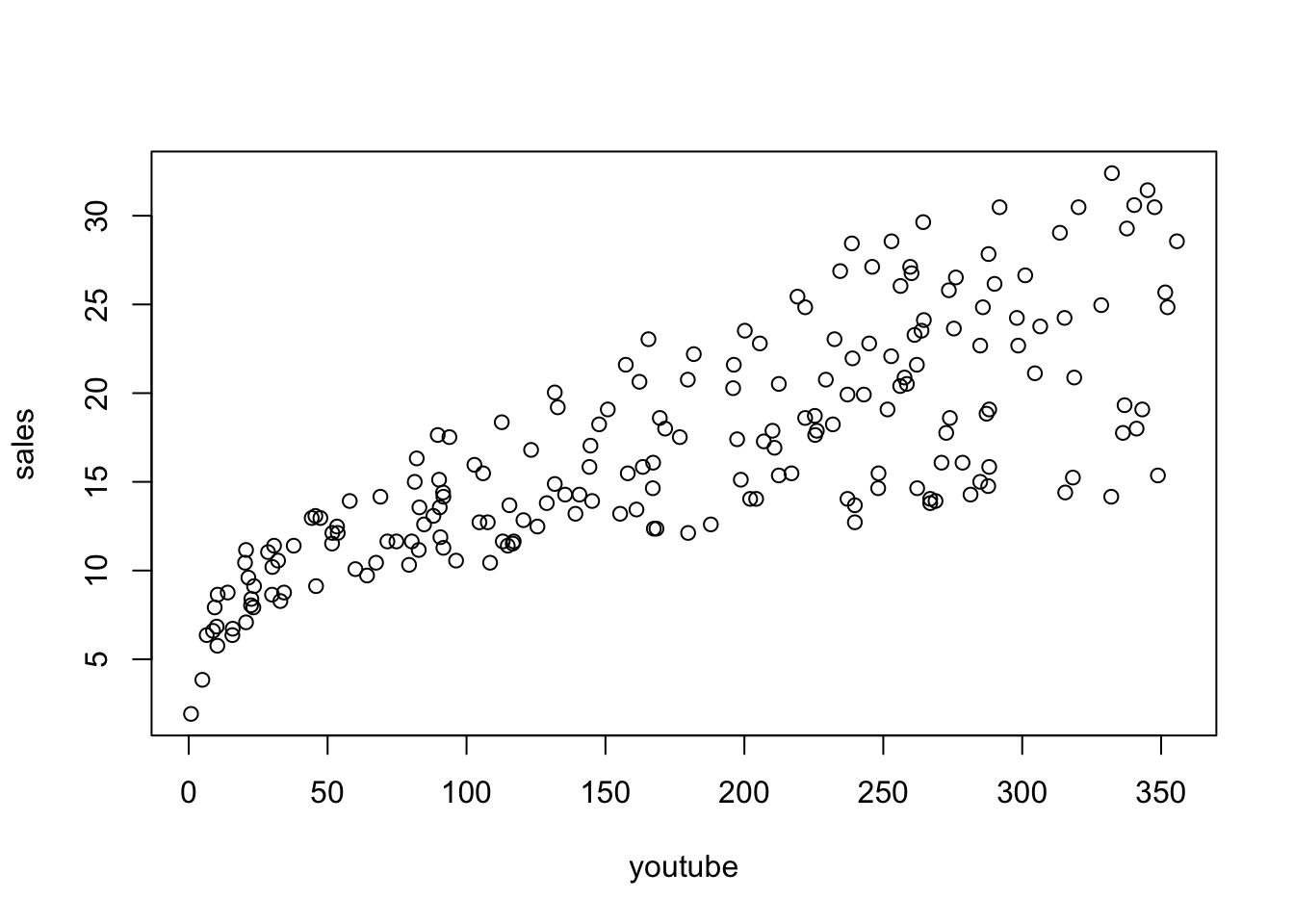

myfit <- lm(sales~youtube, data = marketing)
summary(myfit)


Call:
lm(formula = sales ~ youtube, data = marketing)

Residuals:
     Min       1Q   Median       3Q      Max 
-10.0632  -2.3454  -0.2295   2.4805   8.6548 

Coefficients:
            Estimate Std. Error t value Pr(>|t|)    
(Intercept) 8.439112   0.549412   15.36   <2e-16 ***
youtube     0.047537   0.002691   17.67   <2e-16 ***
---
Signif. codes:  0 '***' 0.001 '**' 0.01 '*' 0.05 '.' 0.1 ' ' 1

Residual standard error: 3.91 on 198 degrees of freedom
Multiple R-squared:  0.6119,    Adjusted R-squared:  0.6099 
F-statistic: 312.1 on 1 and 198 DF,  p-value: < 2.2e-16

plot(sales~youtube, data = marketing)
abline(myfit, col = 2, lwd = 2)

Checking model assumptions

In 2D (as is the case with SLR), we can check all of our assumptions directly on the scatterplot. Not that we could also investigate the following diagnostic plots.

par(mfrow=c(2,2))
plot(myfit)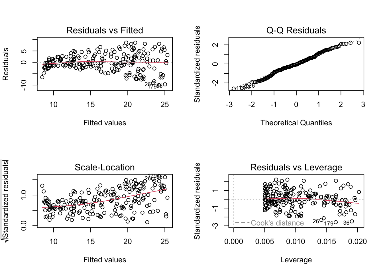

Making Predictions

Given a value of $x$, we can make predictions for $y$, denoted $\hat y$ using the formula:

\[ \hat Y = \hat \beta_0 + \hat \beta_1 x \]

You should know how to extract these values from the summary output of an lm

Chi-squared test for count data

In lecture we investigated two main variants of the $\chi^2$ test for count data:

Goodness of fit test AKA tests for one-way table
Test for Independence AKA tests for two-way table

Goodness of fit test

In tests for one-way tables, observations are classified according to a single categorical variable (with more than 2 levels)

	Level 1	Level 2	Level 3
Observed	$O_1$	$O_2$	$O_3$
Expected	$E_1$	$E_2$	$E_3$

One-way tables: Application: used with one-way tables where there’s a single categorical variable: Goal: To evaluate if the observed frequencies deviate from a hypothesized distribution. \[ \begin{equation} \sum_{i = 1}^{k} \dfrac{(O_i - E_i)^2}{E_i} \sim \chi^2_{df = k-1} \end{equation} \] A high $\chi^2$ value value indicates a poor fit; the data does not follow the hypothesized distribution

Test for Independence

In tests for two-way tables, observations are classified according to a two different categorical variable.

A two-way contingency table² presents the frequency distribution of variables in a matrix format. The rows represent the categories of one variable, while the columns represent the categories of another.

	Category 1	Category 2	Total
Group A	$A$	$B$	$A + B$
Group B	$C$	$D$	$C + D$
Total	$A +C$	$B + D$	$T$

$A, B, C, D$: Number of observations for a specific category combination.
The marginal totals are given in the margins, and represent the total observations in the respective row/column.
$T = A+ B+ C+D$: Total observations in the table.

Two-way tables: Application: used with two-way contingency tables having two categorical variables: Goal: To determine if there is a significant association between the two variables \[ \begin{equation} \sum_{i = 1}^{rc} \dfrac{(O_i - E_i)^2}{E_i} \sim \chi^2_{df = (r-1)(c-1)} \end{equation} \] A high $\chi^2$ value value indicates an association between the variables

To be updated with more details!

Footnotes

Some resources only use a check of $np \geq 5$ and $n(1 - p) \geq 5$↩︎
also known as a cross-tabulation or crosstab or two-way table.↩︎

	Level 1	Level 2	Level 3
Observed	\(O_1\)	\(O_2\)	\(O_3\)
Expected	\(E_1\)	\(E_2\)	\(E_3\)

	Category 1	Category 2	Total
Group A	\(A\)	\(B\)	\(A + B\)
Group B	\(C\)	\(D\)	\(C + D\)
Total	\(A +C\)	\(B + D\)	\(T\)

Exam Format

Post-midterm review

Hypothesis Testing

1. State the Hypotheses:

2. Choose the Significance Level (\(\alpha\))

3. Select a Statistical Test

4. Collect Data and Calculate Test Statistic

5. Determine the Distribution of the Test Statistic

6. Calculate Critical Value or p-value

7. Make a Decision

8. Draw Conclusions

Critical Value Approach

P-value approach

One-sample Hypothesis Tests

Z-tests

Hypothesis test for the mean

Hypothesis Tests for Proportions

t-test

Chi-squared test for variance

Checking the normality assumption

Confidence Intervals

CI for population mean with know population variance

CI for population mean with unknown population variance

CI for population proportion

CI for population variance

Connection between CI and two-sided tests

Two-sample Hypothesis Tests for the mean

Paired t-test

Pooled t-test

Checking for equal Variance

Welch’s Procedure

ANOVA

Pairwise comparisons

Simple Linear Regression

Example

Checking model assumptions

Making Predictions

Chi-squared test for count data

Goodness of fit test

Test for Independence

Footnotes