flowchart TB
  B[Supervised]
  C[Unsupervised]

  C -- Group by similarity --> C1["<div style='text-align: left'><b>Clustering</b><br>- k-means<br>- hclust<br>- GMM</div>"]
  C -- Transform/Reduce --> C2["<div style='text-align: left'><b>Dimension Reduction</b><br>- PCA</div>"]
  B -- Predict a category/number --> H["<div style='text-align: left'>- k-nearest neighbours<br>- Neural Networks<br>- Decision Trees<br><i>Ensemble methods</i><br>- Random Forests<br>- Bagging<br>- Boosting</div>"]


  B -- Predict a category --> F["<div style='text-align: left'><b>Classification</b><br>- logistic regression<br>- LDA/QDA</div>"]
  B -- Predict a number --> G["<div style='text-align: left'><b>Regression</b><br>- OLS Regression<br>- PCA regression <br>- PLS<br><i>Regularization methods</i><br>- Ridge<br>- LASSO</div>"]

  F --> I["<div style='text-align: left'><b>Classification Metrics</b><br>- Confusion Matrix<br>- accuracy<br>- error rate<br>- precision<br>- recall/sensitivity<br>- specificity<br>- F1-score</div>"]


  G --> J["<div style='text-align: left'><b>Regression Metrics</b><br>- MSE<br>- RMSE<br>- MAE<br>- R-squared<br>- Adj. R-squared</div>"]

  H --> K["<div style='text-align: left'><b>Bagging/RF metrics</b><br>- OOB MSE<br>- OOB error rate</div>"]

  C1 --> L["<div style='text-align: left'><b>Group selection</b><br>- scree plot or WSS<br>- jumps in dendogram<br>- BIC</div>"]

  C2 --> M["<div style='text-align: left'><b># of Components</b><br>- Cumulative percent of variance<br>- Kaiser criterion<br>- Scree plot or eigenvalues</div>"]

  F:::Note
  C1:::Note
  C2:::Note
  C:::Ash
  B:::Ash
  G:::Important
  J:::Warning
  I:::Warning
  K:::Warning
  L:::Warning
  H:::Purple
  M:::Warning

  classDef Aqua fill:#DEFFF8, color:#378E7A
  classDef Sky stroke-width:1px, stroke-dasharray:none, stroke:#374D7C, fill:#E2EBFF, color:#374D7C
  classDef Rose stroke-width:1px, stroke-dasharray:none, stroke:#FF5978, fill:#FFDFE5, color:#8E2236
  classDef Note stroke:#a3b8d0, fill:#ecf4fd, color:#4078C0
  classDef Warning stroke:#d24e01, fill: #fff2eb, color:#dc6601
  classDef Important stroke:#FF5978, fill: #ffeaee, color:#8E2236
  classDef Tip fill: #ffeaee, color:#4CAF50
  classDef Caution fill: #ffeaee, color:#000000
  classDef Tip fill: #ffeaee, color:#000000
  classDef Purple fill: #e2d4e8, color:#5D3A8C, stroke: #c0afc8
  classDef Ash stroke-width:1px, stroke-dasharray:none, stroke:#999999, fill:#EEEEEE, color:#000000


linkStyle 0 stroke-width:1px, stroke:black, color:black, background:none;
linkStyle 1 stroke-width:1px, stroke:black, color:black, background:none;
linkStyle 2 stroke-width:1px, stroke:black, color:black, background:none;
linkStyle 3 stroke-width:1px, stroke:black, color:black, background:none;
linkStyle 4 stroke-width:1px, stroke:black, color:black, background:none;
Exam Review
Format
This exam is cumulative.
- On paper - handwritten.
- a mix of multiple choice, and short/long answer
- closed-book, closed-technology
- i.e. computers, smart watches, and calculators are not permitted
- 1 doubled-sided 8.5x11 handwritten formula sheet is allowed
Strikthrough text (e.g. strikethrough text) indicate items that will not be tested on the final.
Overarching Topics
R, RStudio, and Quarto
R and RStudio for statistical analysis.
- R basics, syntax, libraries and installations
- basic data manipulation, summarization, and visualization
- Produce an HTML output from an Rmd file
Quarto
- YAML (e.g.
embed-resources: true) - Markdown basic syntax (
## Level 2 header,**bold**,*italics*) - code chunk options (e.g.
echo: true) code on how to embed an image
- YAML (e.g.
R functions and libraries
- A list of functions and partial help files will be provided as needed on the exam (similar to Midterm 2).
- You should know how to use the functions used throughout the course to implement these techniques.
- Questions will include, MCQ/fill-in-the-blank inputs
- Interpreting R output
Note
In addition to knowing how to use these functions, you should also have a general concept of how they work. You may be asked question on describing (e.g. pseudo code or short description) on an algorithm.
Types of Machine Learning
Workflow for assessment
Preprocessing considerations
- test/train split
- to scale or not to scale
- feature selection
- feature engineering
Notation and Terminology:
- \(X\) = predictors, \(Y\) = response, \(n\) = number of observations, \(p\) = number of predictors
- Supervised (\(X\)’s and \(Y\)’s) vs unsupervised (no \(Y\))
Choosing a Model
Inference vs. prediction
Goal of prediction: is to estimate an outcome or value based on historical data, patterns, and relationships present in the input features. The fundamental idea is to use a model trained on existing data to make informed predictions about unseen or future data.
Goal of inference:
- To gain insights about the underlying data generation process, relationships between variables, or the impact of certain factors.
- To draw conclusions or make statements about the population or data generating mechanism.
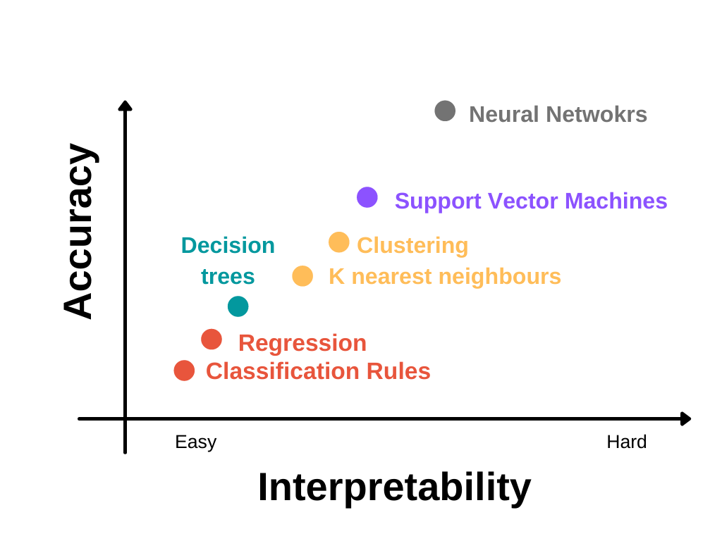
Accuracy vs. Interpretability
Bias-Variance tradeoff
The bias-variance tradeoff suggests that as you decrease bias (by using a more complex model), you often increase variance, and vice versa. The challenge is to find the right level of model complexity that minimizes the total error on unseen data. The complexity of a model is often controlled by hyperparameters or features such as the degree of a polynomial, the depth of a decision tree, or the number of parameters in a neural network.
\[ \text{Total Error} = \text{Bias}^2 + \text{Variance} + \text{Irreducible Error} \]
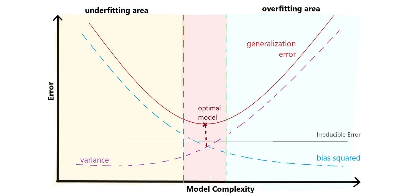
The U-shaped test MSE (generalization error in this visualization) is a fundamental property of statistical learning that holds regardless of the particular dataset and statistical method being used.
Bias (Model Error):
Definition: Bias is the error introduced by approximating a real-world problem with a simplified model. It represents the difference between the predicted values of the model and the true values.
Effect: High bias models tend to oversimplify the underlying patterns in the data, leading to systematic errors.
Relation to Model Complexity: Bias is often associated with models that are too simple or have insufficient capacity to capture the complexity of the underlying relationship in the data.
Variance (Model Sensitivity):
Definition: Variance is the error introduced by the model’s sensitivity to the fluctuations in the training data. It measures how much the model’s predictions vary when trained on different subsets of the data.
Effect: High variance models fit the training data too closely and may not generalize well to new, unseen data.
Relation to Model Complexity: Variance is often associated with models that are too complex, capturing noise or specific patterns in the training data that do not generalize.
Irreducible Error:
Definition: Irreducible error is the error that cannot be reduced by any model. It stems from the inherent randomness or noise in the data, and it represents the minimum error that any predictive model will have.
Effect: No matter how accurate a model is, there will always be some level of error that cannot be eliminated.
Relation to Total Error: Irreducible error sets a lower limit on the total error that any model can achieve. It is the baseline level of error that even an optimal model cannot overcome.
Total Error:
Definition: Total error is the sum of the squared bias, variance, and irreducible error.
Relationship: The bias-variance tradeoff illustrates that as you reduce bias, variance tends to increase, and vice versa. The total error of a model is the sum of the squared bias, variance, and irreducible error.
\[ \text{Total Error} = \text{Bias}^2 + \text{Variance} + \text{Irreducible Error} \]
The goal is to find a model complexity that minimizes the total error by balancing bias and variance. Achieving zero bias and zero variance is typically not possible, and the tradeoff involves finding the right level of complexity.
Underfitting vs overfitting
Underfitting (High Bias): Occurs when a model is too simple to capture the underlying patterns in the data. It performs poorly on both the training and new data.
Overfitting (High Variance): Occurs when a model is too complex and fits the training data too closely. It performs well on the training data but poorly on new, unseen data.
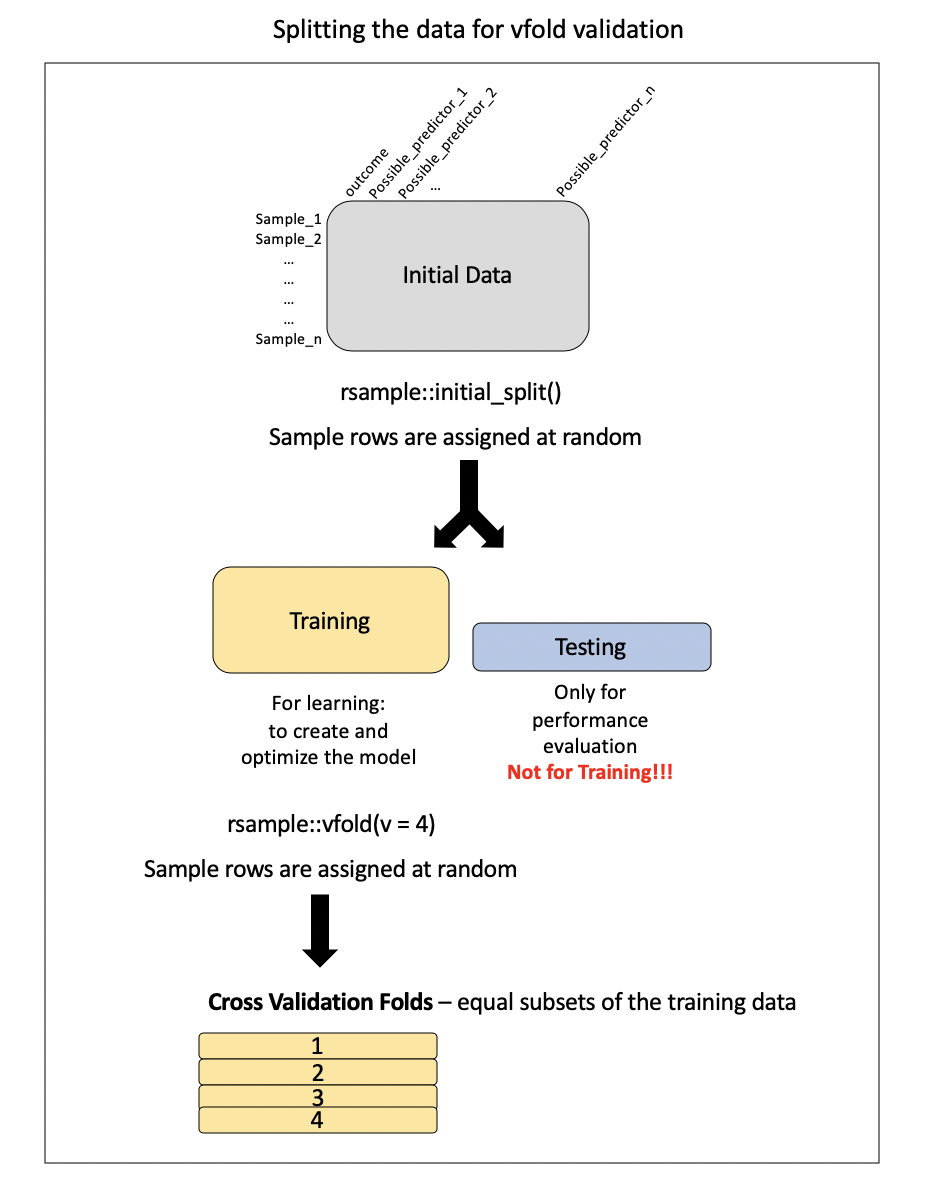
Resampling methods
Both cross validation and bootstrapping are resampling methods.
- CV is often used to help select a model (also know as tuning a model)
- The bootstrap is often used to quantify the uncertainty associated with a given estimator or statistical learning method.
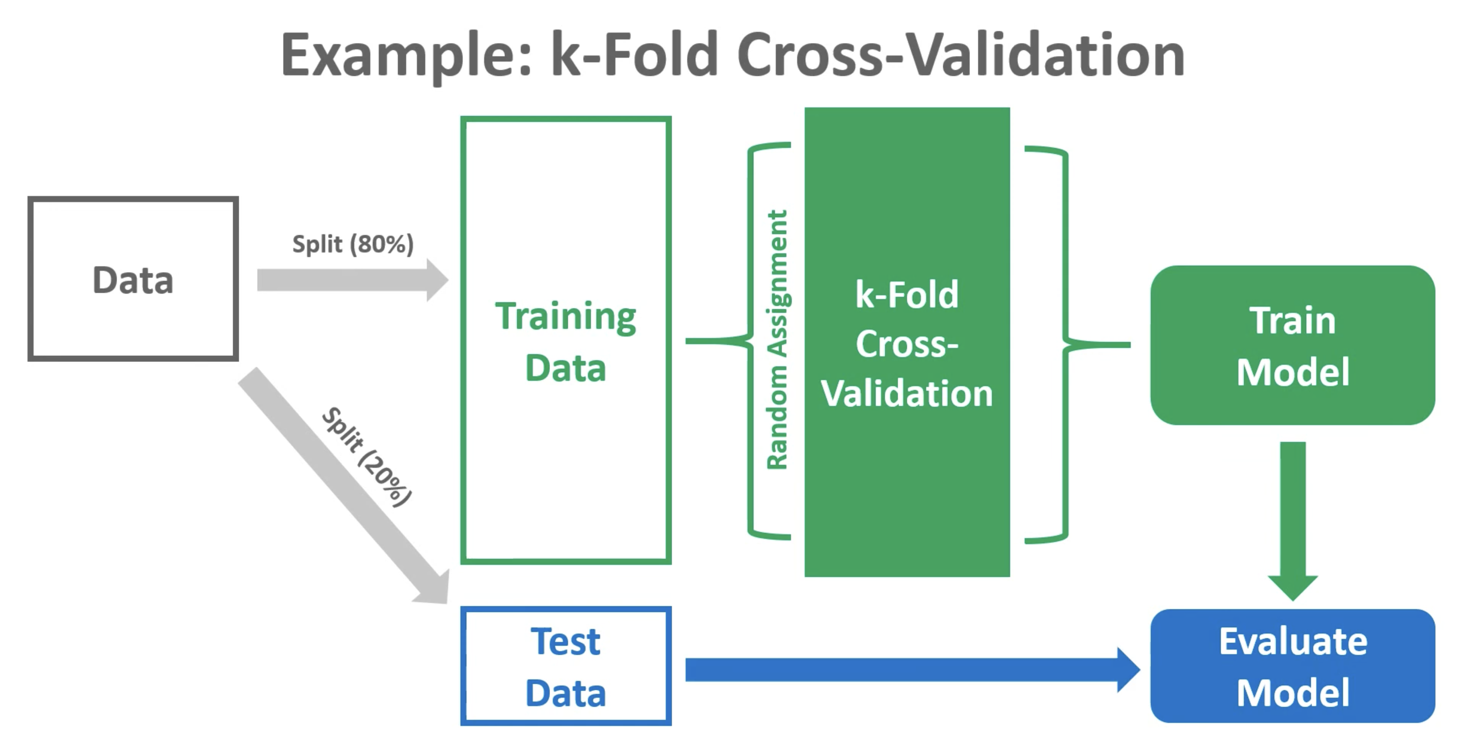
Cross-validation
Training may involve model tuning. Model tuning with cross-validation is a crucial step in the machine learning pipeline to optimize the performance of a model by adjusting hyperparameters. Hyperparameters are settings that are not learned from the data but need to be specified before the training process. Cross-validation is used to assess different hyperparameter options and choose the value with the best generalization performance. Here’s how it works:
Hyperparameter Selection:
Choose a set of candidate hyperparameters for your machine learning model. These might include parameters like the depth of a decision tree, \(k\) = the number of nearest neighbours to be used in KNN, the regularization parameter \(\alpha\) in LASSO/Ridge regression, …
Cross-Validation Setup:
Model Training and Evaluation:
For each candidate value for you hyperparameter:
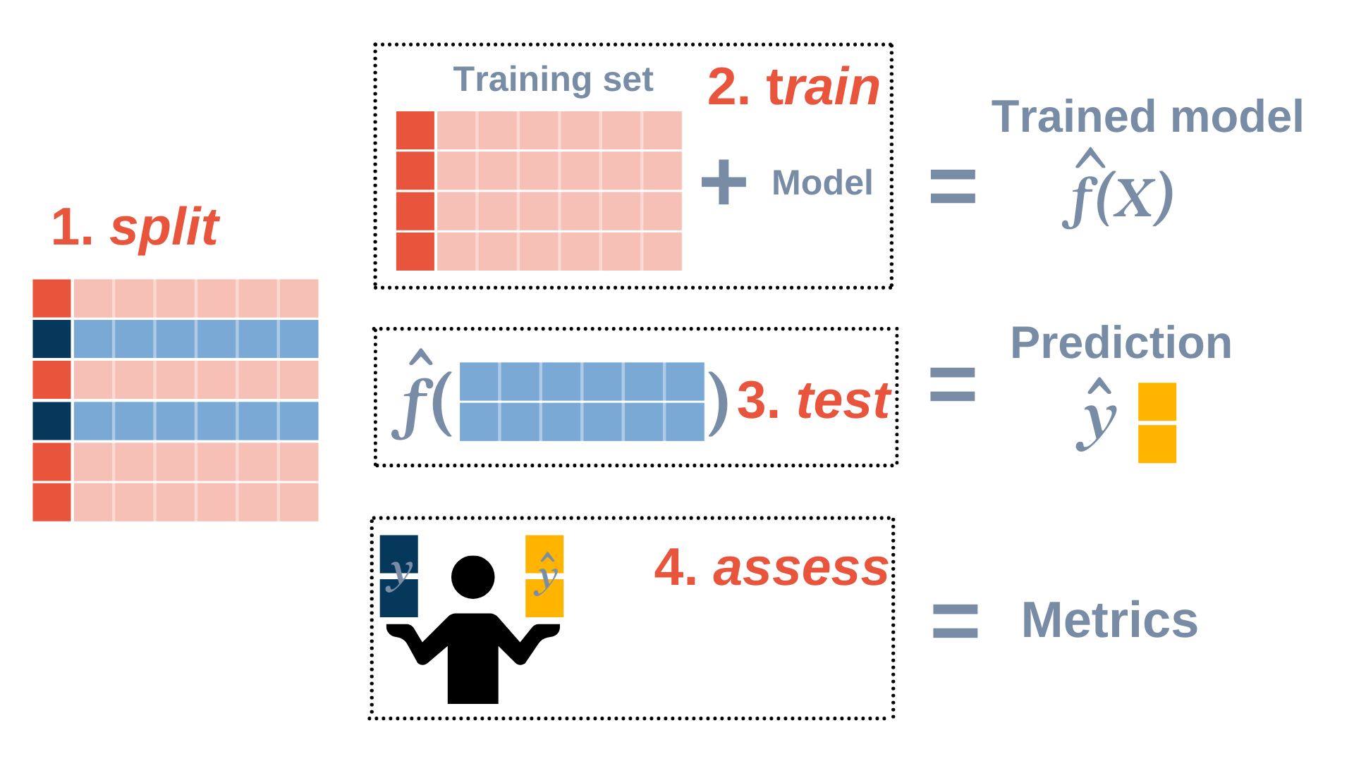
Train the model on the training subset with the chosen hyperparameters. See Figure 2.
Evaluate the model’s performance on the validation subset using a predefined metric (e.g., accuracy, precision, recall). See Figure 2.
Compute the average performance across all folds to get a more reliable estimate of the model’s generalization performance with the current hyperparameter settings.
Final Model Selection:
- Refit the model with the choosen hyperparameter value that resulted in the best average performance across all folds.
Final Model Assessment
- For a more robust assessment, perform a final evaluation on a separate test set that wasn’t used during hyperparameter tuning.

Bootstrap
Bootstrapping is a resampling procedure that resamples a single data set (with replacement) to create many multiple “bootstrap samples”.
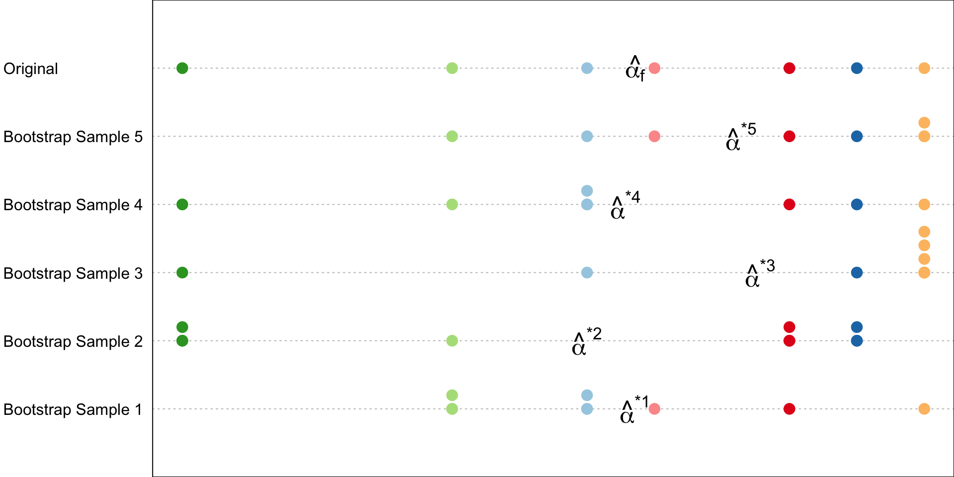
This process allows us to assess the variability of a statistical estimator or to improve the robustness of a machine learning model. Here’s how we saw bootstrap in use:
Estimation of standard errors and confidence intervals: bootstrap resampling can be used to estimate stanadard errors and confidence intervals around model parameters. By repeatedly resampling the dataset and fitting the model, you can assess the variability of the estimated parameters. Know how to read/write a program for doing this.
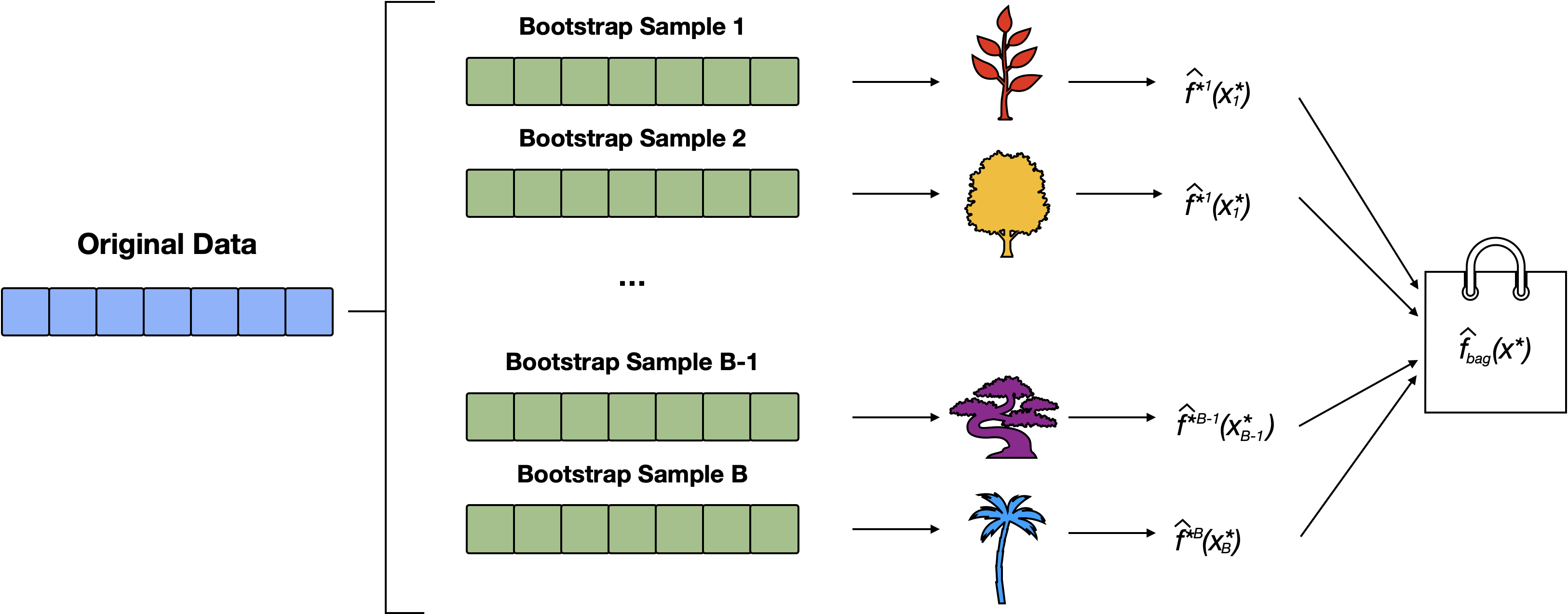
Bagging (Bootstrap Aggregating): the bootstrap can be employed in ensemble methods like bagging decisions trees. More generally bagging involves training multiple instances of the same learning algorithm on different bootstrap samples of the training data and combining their predictions to reduce variance and improve generalization.
Random Forests: (an extension of Bagging, where each tree is constructed using a random subset of features at each split, introducing an additional layer of randomness) used bootstrap sampling to create multiple decision trees. Each tree is trained on a bootstrap sample, and their predictions are combined through voting or averaging.
Feature Importance: In bagging and random forests the bootstrap inherently provides an estimate the importance of features in a model. The importance is infered by assessing how the model performance changes with and without each feature.
Out-of-bag error estimates: In ensemble methods like Random Forests and Bagging, out-of-bag (OOB) estimates of error provide a way to assess the model’s performance without the need for a separate validation set or cross-validation. Here’s how it works:
During the training of each tree in the ensemble, a bootstrap sample (a random sample with replacement) is drawn from the original dataset; the instances from the training set that are not sampled are called the “out-of-bag” samples.
For each observation in the training set we predict its target variable using only the trees for which it was an out-of-bag sample and calculate the error (e.g., classification error or mean squared error).
Steps
Consider some estimator \(\hat \alpha\). For \(j = 1, 2, \dots B\) 1
- take a random sample of size2 \(n\) from your original data set with replacement. This is the \(j\)th bootstrap sample, \(Z^{*j}\)
- calculate the estimated value of your parameter from your bootstrap sample, \(Z^{*j}\), call this value \(\hat \alpha^{*j}\).
Estimate the standard error and/or bias of the estimator, \(\hat \alpha\), using the equations given on the upcoming slides.
Bootstrap Standard Error
Bootstrap estimates the standard error of estimator \(\hat \alpha\) using3
\[\begin{equation} \hat{\text{SE}}(\hat \alpha) = \sqrt{\frac{\sum_{i=1}^{B} (\hat \alpha^{*i} - \overline{\hat \alpha})^2}{B -1}} \end{equation}\]
where \(\overline{\hat \alpha} = \sum_{j = 1}^B \hat \alpha^{*j}\) is the average estimated value over all \(B\) bootstrap samples.
Bootstrap Bias
The bootstrap estimates the Bias of estimator \(\hat \alpha\) using:
\[\begin{align} \hat{\text{Bias}}(\hat \alpha) = \overline {\hat \alpha} - \hat \alpha_f \end{align}\]
where \(\overline{\hat \alpha} = \sum_{j = 1}^B \hat \alpha^{*j}\) and \(\hat \alpha_f\) is the estimate obtained on the original data set.
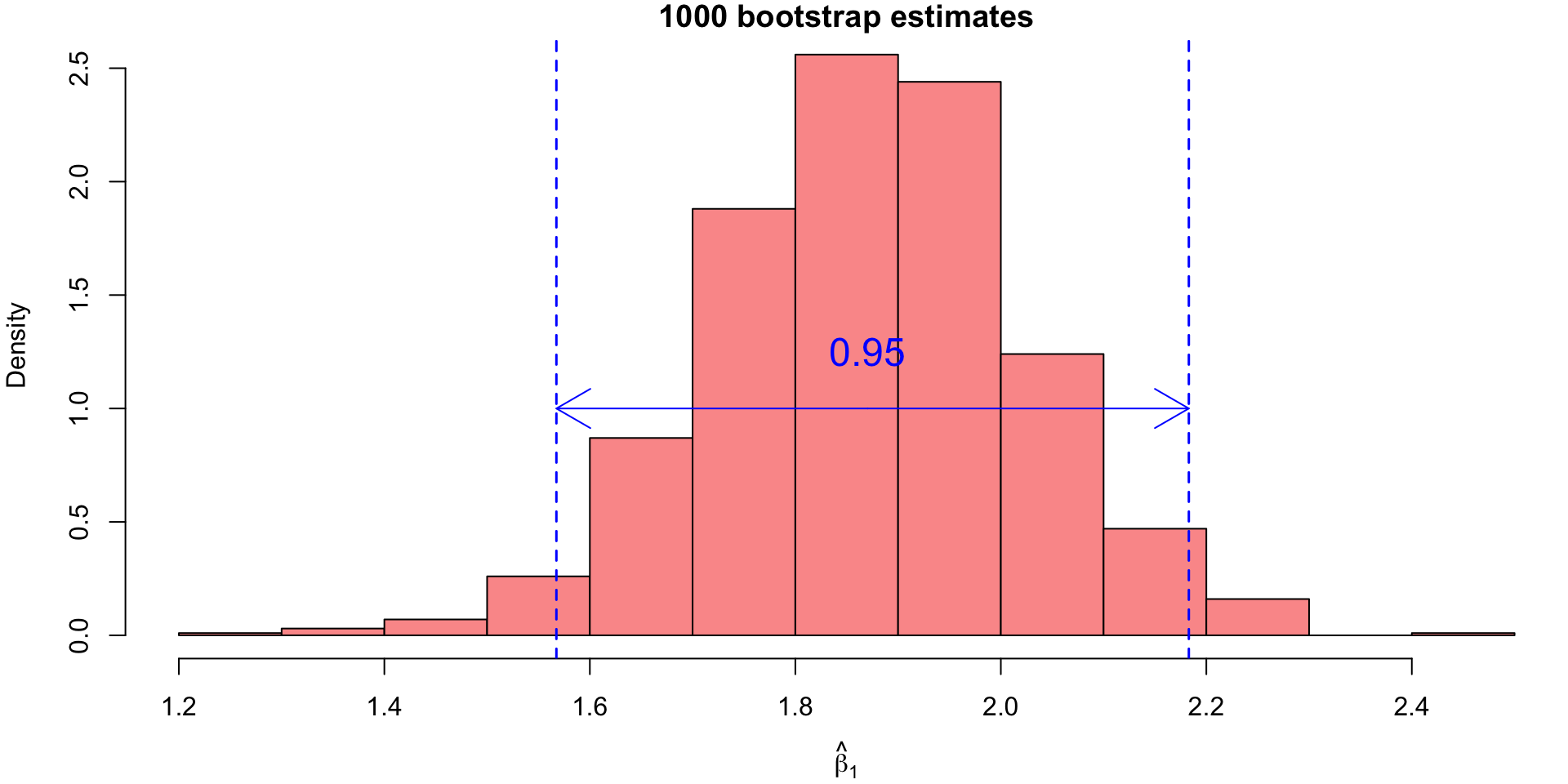
Bootstrap Confidence Intervals (CI)
- To obtain confidence intervals from this empirical distribution, we would simply finding appropriate percentiles.
- For our example, the 95% bootstrap CI for \(\beta_1\) would correspond to the 25th value and the 975th value of the sorted bootstrap estimates.
Metrics for Assessment
Metrics for Regression
Mean Squared Error (MSE) and Training vs. Testing MSE.
\[ MSE = \frac{1}{n} \sum_{i=1}^{n} (y_i - \hat{y}_i)^2 \]
we typically care more about the MSE calculated on the test set. Some general trends:
- As model flexibility increases, the training MSE will decrease, but the test MSE may not.
- When a method yields a small training MSE but a large test MSE, is is said to be overfitting the data.
- We almost always expect the training MSE to be smaller than the test MSE.
- The training MSE declines monotonically as flexibility increases.
Metrics for Classification
We often look at confusion matrices that have the form:
Confusion Matrix
| Predicted Yes | Predicted No | |
|---|---|---|
| Actual Yes | TP = True Positive | FN = False Negative |
| Actual No | FP = False Positive | TN= True Negative |
Accuracy: \(\frac{\text{True Positives} + \text{True Negatives}}{\text{Total Population}}\)
Precision (Positive Predictive Value): \(\frac{\text{True Positives}}{\text{True Positives} + \text{False Positives}}\)
Recall (Sensitivity, True Positive Rate): \(\frac{\text{True Positives}}{\text{True Positives} + \text{False Negatives}}\)
F1 Score: \(2 \times \frac{\text{Precision} \times \text{Recall}}{\text{Precision} + \text{Recall}}\)
Primary Measures
From the confusion matrix we can extract things like:
Misclassifcation (aka error) rate: \(\frac{FP + FN}{\text{Total number of predictions}}\)
Accuracy: \(\frac{TP + TN}{\text{Total number of prediction}}\)
Accuracy can sometimes be a misleading measure (especially with umbalanced4 data). Other metrics we can consider are:
Precision: \(\frac{TP}{TP + FP}\) = proportion of predicted Yes’ that are actually Yes.
- e.g. good for spam detection
Recall (aka sensitivity): \(\frac{TP}{TP + FN}\) the proportion of actual Yes’ that were predicted Yes.
- e.g good for disease diagnostic
Specificity: \(\frac{TN}{TN + FP}\) the proportion of actual No’s that were predicted No.
- e.g. good for quality control
F1
Another useful/common metric is the F1 score. It is the harmonic mean between Precision and Recall.
\[ \text{F1} = \dfrac{2 \times \text{Precision} \times \text{Recall}} {\text{Precision} + \text{Recall}} \]
This is a value between 0 and 1 (0 being the worst score, 1 being the best score). In practical scenarios, the F1 score typically falls between 0 and 1. Values closer to 1 indicate better balance between precision and recall, while values closer to 0 suggest an imbalance or trade-off between precision and recall.
Note: while the F1 score is simplest to explain in the binary classification problem, it can be used in the multiclass scenario as well (details not provided).
The harmonic mean is particularly useful in situations where extreme values (e.g., one of precision or recall being very low) should heavily impact the overall score.
# Example data
precision <- 0.9
recall <- 0.1

hmean <- function(p,f) { 2*p*f/(p+f)}

# Calculate the harmonic mean (F1 score)
hmean(precision, recall)
[1] 0.18mean(c(precision, recall))[1] 0.5F1 score is at its minimum when either precision or recall is zero.
- This occurs when all predictions are incorrect for one of the classes (e.g., no true positives for recall or no true positives for precision). In such cases, the F1 score approaches 0.
The F1 score is at its maximum value of 1 when both precision and recall are perfect.
Supervised Learning
Statistical Learning Model
\[Y = f(X) + \epsilon\] Statistical learning is concerned with estimating \(f\). Estimates of \(f\) are denoted by \(\hat f\), and \(\hat y\) will represent the resulting prediction for \(y\).
General workflow:
Regression/Classification Models
We saw a collection of models that could be used for both regression regression.
K-Nearest Neighbors (KNN):
- Model: This is a a non-parametric technique that predicts the continuous output/class based on the average/majority vote of the k-nearest neighbors in the feature space.
- Objective: Captures local patterns in the data.
- Use Cases: Suitable for problems where local relationships are important and the data has a clear structure. Simple and intuitive, suitable for both binary and multiclass classification.
- Choice of \(k\)
- possible values are 1,…, \(n\)
- A small \(k\) : High variance (sensitive to noise).
- A large \(k\) : High bias (can smooth over local patterns):
- Choosen using cross-validation (choose the \(k\) that minimizes CV-error / maximizes accuracy)
- Practical considerations
- Range of \(k\) (nearest neighbor) and go up to a reasonable fraction of the dataset size (e.g., \(k = 1, \dots, \sqrt{n}\)
- Avoid very large \(k\) as it approaches global averaging and becomes less meaningful.
- Prefer odd values of \(k\) for binary classification to avoid ties in voting
- If cross-validation suggests that the best kkk lies at the boundary of your search range, expand the search range
Neural Networks
- Neural Networks are a set of algorithms modeled after the human brain, designed to recognize patterns and learn relationships from data.
- Captures complex relationships that linear models cannot.
Basic Architecture:
They consist of interconnected nodes (neurons) organized into layers: an input layer, one or more hidden layers, and an output layer.
Neurons:
Basic units that take weighted inputs, apply an activation function, and output a value.
Similar to biological neurons.
Layers:
Input Layer: Takes input features.
Hidden Layers: Perform intermediate computations.
Output Layer: Produces the final output (e.g., class probabilities or regression value).
Weights and Biases:
The connections between nodes are characterized by weights, which are adjusted during training to capture the relationships in the data.
Biases are additional parameters that allow the model to account for shifts in the data.
Activation Function:
- Each node in a neural network applies an activation function to its input.
- Common activation functions include sigmoid, hyperbolic tangent (tanh), and rectified linear unit (ReLU).
Tuning a NNet
Feedforward: During the training process, input data are fed forward through the network, and predictions are compared to the actual outcomes
Backpropagation involves calculating the gradient of the loss function with respect to each weight and bias.
Stochastic Gradient Descent is commonly used to calculate the gradient of the loss function based on individual samples or mini-batches of data.
One complete pass through the entire training dataset (including feedforward, backpropagation, and weight updates) is called an epoch
Loss Function:
- A loss function quantifies the difference between predicted and actual values. During training, the goal is to minimize this loss.
- Mean Squared Error (for regression).
- Cross-Entropy Loss (for classification).
Extension to the single-layer neural network we looked at in class:
Deep learning extends neural networks to include multiple hidden layers, leading to the term “deep neural networks.”
Convolutional Neural Networks (CNNs): Specialized architectures for image-related tasks. CNNs use convolutional layers to automatically learn spatial hierarchies of featuresRecurrent Neural Networks (RNNs): Suited for sequential data. RNNs maintain a hidden state that captures temporal dependencies in sequencesRegularization (L1/L2, or dropout)
You should know:
how to read a network diagram and determine the number of parameters
key terms (e.g. whats a epoch)
key concepts (e.g. why would we consider regularization techniques and what do these methods do)
Tree-based methods
Tree-based methods are used in both regression and classification tasks, making them versatile and widely applicable in machine learning. We generally would expect CART < Bagging < Random Forests for more complicated problems.
Classification and Regression Trees (CART)
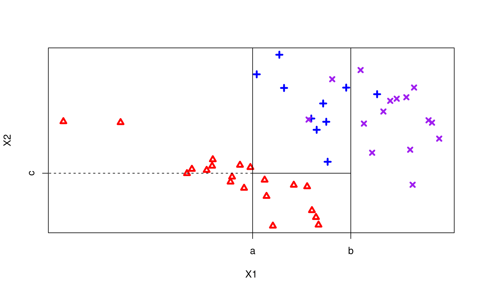
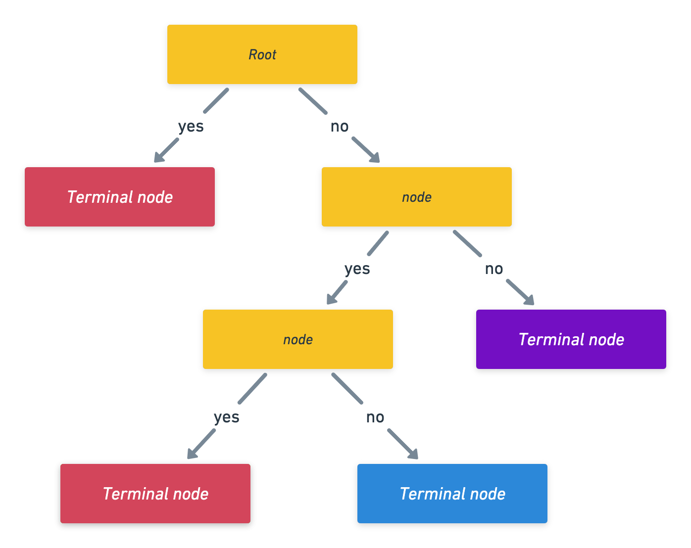
Classification and Regression Trees (AKA CART or decision trees) involve partitioning (AKA stratifying or segmenting) the predictor/feature space by simple binary splitting rules.
Model: Builds a tree structure to make predictions based on recursive binary splits of the input features. Each internal node represents a decision, and each leaf node represents the prediction (e.g. value or class label).
Objective (for classification): The goal of a decision tree for classification is to partition the input space into distinct regions, each corresponding to a specific class or category. Maximizes information gain or Gini impurity during tree construction.
Objective (for regression): Minimize the RSS (via recursive binary splitting) at each node.
Use Cases: Versatile for both binary and multiclass classification. Interpretability is a notable advantage. Suitable for problems with complex, non-linear relationships. Prone to overfitting.
Pruning: technique used to prevent overfitting by removing or merging nodes.
Since the set of splitting rules used to segment the predictor space can be summarized in a tree, these types of approaches are known as decision tree methods.
We make a prediction for an obs. using the mean/mode response value for that “region” to which it belongs.

Notation:
Growing a tree
- First we grow a tree using recursive binary splitting until some stopping criterion in met.
- regression uses RSS for this
- classicifcation grows using the Gini index
- Prune the tree: since the tree in the last time is probably too bushy and has high variance we trim it back using cross-complexity pruning. (use cross-validation to determine by how much)
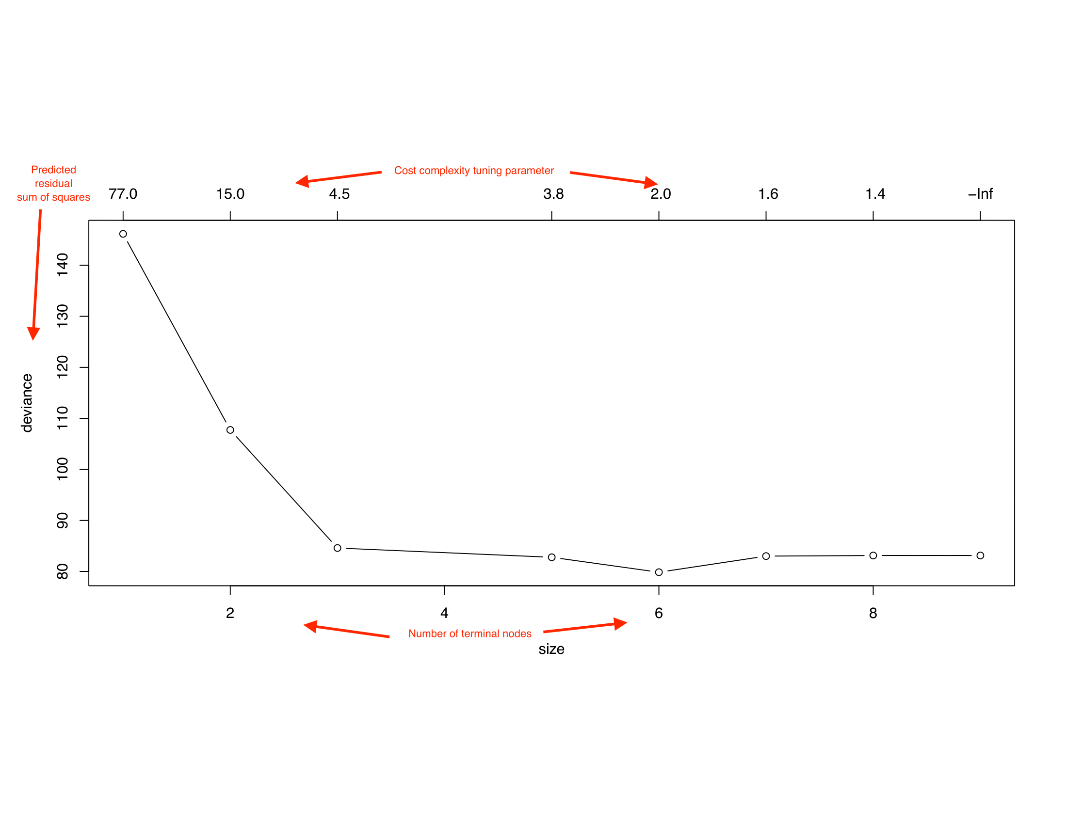
We consider a sequence of trees indexed by a non-negative tuning parameter \(\alpha\). For every value of \(\alpha\) there corresponds a subtree, \(T \in T_0\), such that the following is minimized: \[\begin{equation} \sum_{m=1}^{|T|} \sum_{i:x_i \in R_m} (y_i - \hat y_{R_m})^2 + \alpha |T| \end{equation}\]
- Here \(|T|\) is the number of terminal nodes in the tree,
- \(R_m\) is the region corresponding to the \(m\)th terminal node
- \(\hat y_{R_m}\) is the mean of the training observations in \(R_m\).
Tuning Parameter
- When \(\alpha = 0\), then the subtree \(T\) will simply equal \(T_0\)
- However, as \(\alpha\) increases, there is a price to pay for having a tree with many terminal nodes, and so the penalized RSS will tend to be minimized for a smaller subtree.
- In that way, \(\alpha\) controls the trade-off between the subtree’s complexity and its fit to the training data.
- The tuning parameter \(\alpha\) is selected using cross-validation.
Trees have one aspect that prevents them from being ideal tool for predictive learning, namely inaccuracy. (ESL)
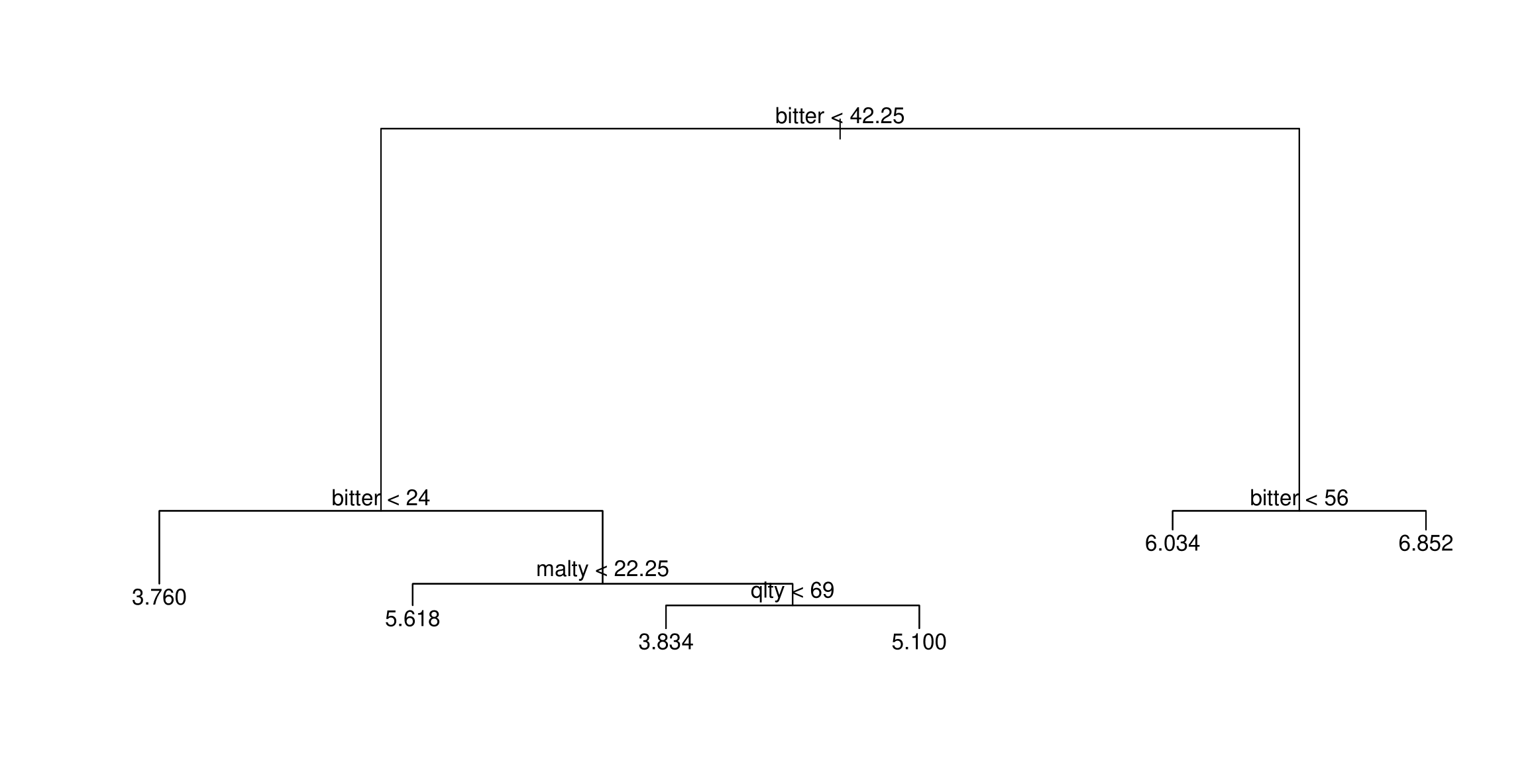
R functions:
tree,cv.tree,prune.treefrom the tree packageKnow how to read the trees and make predictions from them
Bagging and Random Forests
Bagging can be used to improve simple CART by reducing its variance.
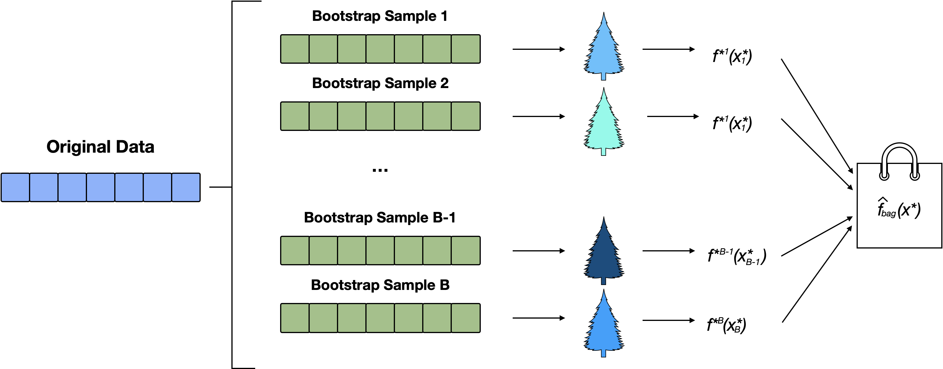
Steps for Bagging
- Create \(B\) bootstrap samples1
- Fit a (bushy) tree to each bootstrap sample
- Each decision tree is used to make a prediction.
- Aggregate the \(B\) predictions:
- for regression predictions are typically averaged
- for classification we use a majority vote.
Random Forest
Random Forests uses a similar method to bagging, however, we only consider m predictors at each split
- default for classification is \(m = \sqrt{p}\)
- default for regression is \(m = p/3\)
Objective: Extend bagging by introducing additional randomness through random feature selection at each split during the construction of decision trees.
Benefits:
- Further reduction of overfitting compared to bagging.
- Improved generalization and accuracy.
Steps for RF
- Create \(B\) bootstrap samples
- Fit a tree to each bootstrap sample, HOWEVER, when creating nodes in each decision tree, only a random subset of \(m\) features is considered for splitting at each node.
- Each decision tree is used to make a prediction. Aggregate the \(B\) predictions.
This modification reduces the variance even more than bagging which tend to improve performance.
Both are fit with the same function in R:
randomForest(formula, data=NULL, mtry, importance = FALSE)when
mtry= \(p\) we get bagging and whenmtry\(< p\) we get random forests. Note that the default values are different for classification (\(\sqrt(p)\) where \(p\) is number of predictors) and regression (\(p/3\))when
importance = TRUEwe get variable importance computations (don’t worry about how they are calculated)
Model assessment
- The out-of-bag (OOB) samples (approximately 1/3 of the data) are used to create an cross-validation like estimate of error
- These are outputted by the
randomForest()function
Pro:
- this approach prevents the risk of overfitting
- we get OOB error estimates “for free”
- makes trees a competitive ML algorithm
- Increased robustness and stability over single Classification decision tree.
- Improved generalization by reducing variance.
- Feature importance analysis.
Con:
- we’ve lost all interpretability
- takes longer to run
Boosting
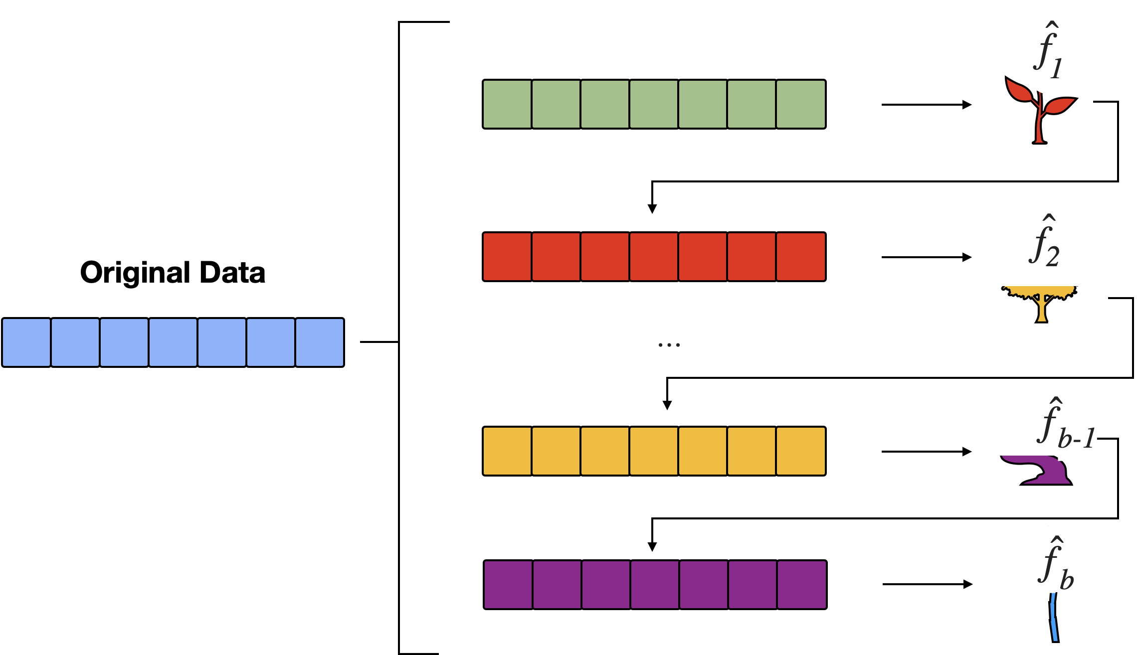
Definition: Boosting is an ensemble learning method that combines the strengths of multiple weak learners to create a strong predictive model.
Objective: Build a strong predictive model by sequentially training weak learners (typically shallow trees), with each new learner focusing on correcting the errors of the ensemble so far.
Key Concepts
Weak Learner: A model that performs slightly better than random guessing. Decision stumps (one-level decision trees) are common weak learners.
Strong Learner: A composite model that achieves high accuracy by aggregating multiple weak learners.
Sequential Learning: Models are trained one after another, with each new model emphasizing the mistakes of the previous ones.
Steps for Boosting
Initialization: Start with a base model (e.g., a simple decision tree) and assign equal weights to all training samples.
Iterative Training:
Training: Train a weak learner on the weighted data.
Evaluation: Assess the learner’s performance and calculate its error rate.
Weight Update: Increase the weights of misclassified instances to focus the next learner on harder cases.
Aggregation: Combine the learners’ predictions, typically using a weighted majority vote (classification) or weighted sum (regression).
Final Model: The ensemble of all weak learners, weighted by their accuracy, forms the final strong model.
Advantages of Boosting
Improved Accuracy: Combines multiple models to achieve higher predictive performance.
Flexibility: Can be applied to various types of models and loss functions.
Handling Complex Patterns: Effective in capturing intricate relationships in data.
Reduction of Bias and Variance: Balances the trade-off between bias (underfitting) and variance (overfitting).
Disadvantages of Boosting
Sensitivity to Noisy Data: Boosting can overemphasize outliers and noisy instances, leading to overfitting.
Computationally Intensive: Especially with large datasets and numerous iterations.
Requires Careful Tuning: Hyperparameters such as the number of learners, learning rate, and tree depth need to be optimized
No more OOB estimates or variable importance
Boosting vs. Bagging
Boosting:
Approach: Sequential training; focuses on correcting errors of previous models.
Goal: Reduce both bias and variance.
Bagging (Bootstrap Aggregating):
Approach: Parallel training on different subsets of data; aggregates predictions.
Goal: Primarily reduce variance; less effective in reducing bias.
Key Difference: Boosting emphasizes sequential improvement, while bagging emphasizes parallel diversity.
Hyperparameter Tuning in Boosting
Number of Estimators: Determines the number of weak learners to combine.
Learning Rate: Controls the contribution of each learner; lower rates require more learners.
Tree Depth: Limits the complexity of each weak learner; deeper trees can capture more complex patterns but may overfit.
Regularization Parameters: Techniques like shrinkage, subsampling, and column sampling to prevent overfitting.
R functions:
gbm(formula, distribution="bernoulli", n.trees = B, interaction.depth = d , shrinkage = lambda)from the gmb package. General expectation of performance:
\[\text{Single Tree} < \text{Bagging} < \text{RF} < \text{Boosting}\]
Regression Models
Regression methods in machine learning are a set of techniques used to model and analyze the relationships between a dependent variable (AKA the target or response variable) and one or more independent variables (AKA features or predictors). The goal is to be able to predict the value of the dependent variable based on the values of the independent variables. Regression models are widely used for both prediction and understanding the underlying relationships within the data. Here are the regression methods we talked about in the course:
Linear Regression
Model: Assumes a linear relationship between the input features and the output. The model is represented as
\[\begin{equation}Y = \beta_0 + \beta_1 X_{1} + \beta_2 X_{2} + \dots + \beta_n X_n \epsilon\end{equation}\]
- \(Y\) is the response variable at \(i\)
- \(X_{j}\) is the \(j^{th}\) predictor variable
- \(\beta_0\) is the intercept (unknown)
- \(\beta_j\) are the regression coefficients (unknown)
- \(\epsilon\) is the error, assumed \(\epsilon_i \sim N(0, \sigma^2)\).
Objective: Minimizes the sum of squared differences between predicted and actual values.
Use Cases: Suitable for problems where the relationship between variables is approximately linear.
Assumptions
Linearity: The relationship between the independent and dependent variables is assumed to be (approximately) linear in the coefficients.
Errors should follow \(\epsilon \sim N(0, \sigma)\)
- The errors (or equivalently observations) should be independent of each other
- The errors term has a population mean of zero.
- Homoscedasticity: the variance of the residuals is constant across all levels of the predictors (no heteroscedasticity)
Multicollinearity
We cannot fit the OLS model when we have perfect multicollinearity5 . When we have multicollinearity in our data, note that regression coefficients
Extending the OLS model
We saw how we could include:
- interaction terms (e.g. \(X_1*X_2\)) to account for scenarios where the impact of one predictor on the response depends on the level or condition of another predictor.
- categorical predictors (by creating dummy variables)
- higher order terms e.g. (\(X_1^3\)) as a way of introducing curvature to capture more complex patterns in the data (polynomial regression)
Feature Selection
For feature selection we could use:
- forward/backwards step-wise selection
- choose the model with the highest adjusted \(R^2\) among some candidate of models
- cross-fold validation (we never did this but hopefully you can visualize how that makes sense)
- use importance features from tree-based models
Be sure to know how to:
- write down the fitted equation of the line(s) from R output
- calculate predictions using R code or by a mathematical equation (final calculation not possible since you are not permitted a calculator)
- read and interpret p-values
- read and interpret R-squared values
lm()functionsummary(lmoutput)
You will not need to know how to:
derive the OLS estimators
Checking Assumptions
Diagnostic Plots
Residuals vs Fitted: checks for linearity. A “good” plot will have a red horizontal line, without distinct patterns.
Normal Q-Q: checks if residuals are normally distributed. It’s “good” if points follow the straight dashed line.
Scale-Location: checks the equal variance of the residuals. “Good” to see horizontal line with equally spread points.
Residuals vs Leverage: identifies influential points.
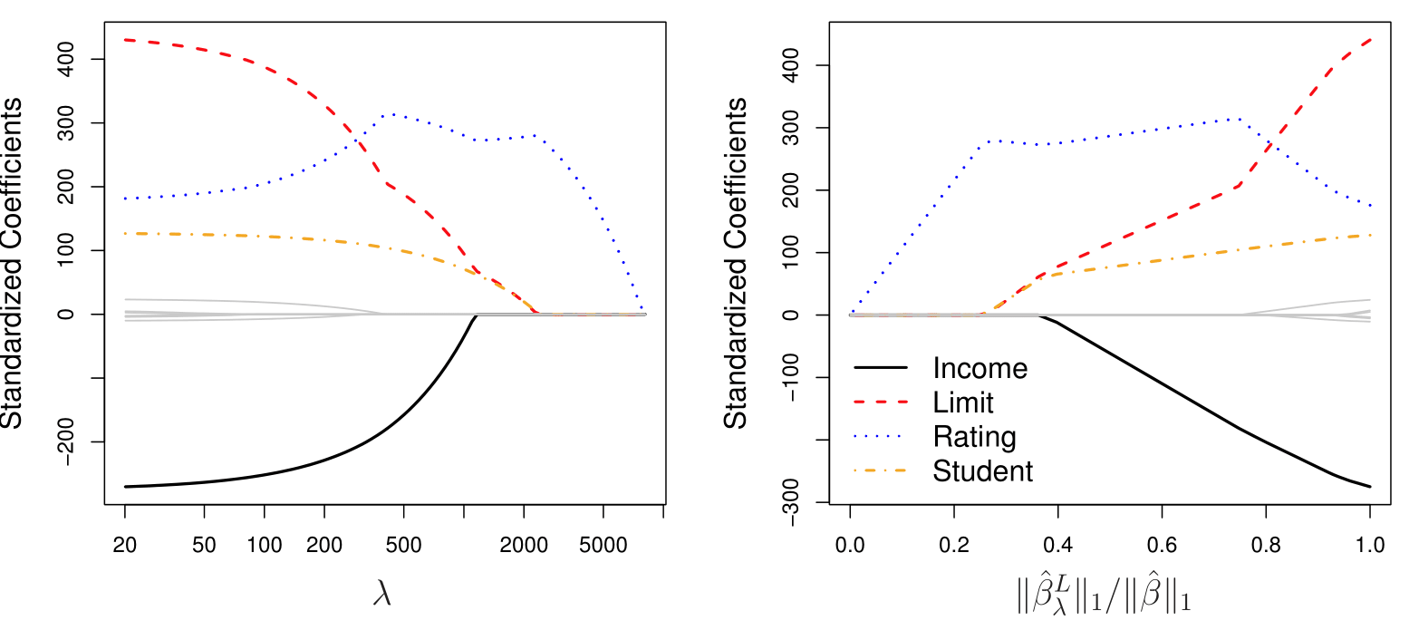
Regularization techniques
Ridge Regression and LASSO (Least Absolute Shrinkage and Selection Operator) are regularization techniques used in linear regression to prevent overfitting and handle multicollinearity. Both methods add a regularization term to the linear regression objective function, influencing the model coefficients during training.
Ridge Regression (L2 Regularization):
Model: A regularized version of linear regression that adds a penalty term proportional to the square of the magnitude of the coefficients.
Objective: Minimizes the sum of squared differences with the addition of a regularization term.
\[ \text{Minimize } \mathcal{L}(\beta) = \sum_{i=1}^{N} (y_i - \beta_0 - \sum_{j=1}^{p} x_{ij}\beta_j)^2 + \lambda \sum_{j=1}^{p} \beta_j^2 \]
Regularization Term: \(\lambda \sum_{j=1}^{p} \beta_j^2\)
Purpose:
Prevents overfitting by shrinking large coefficients, particularly useful when multicollinearity is present.
Does not lead to exact zero coefficients; instead, it shrinks all coefficients proportionally.
Effect on Coefficients:
- Shrinks coefficients closer to zero but does not set any coefficients exactly to zero.
- Does not perform feature selection directly.
Hyperparameter: \(\lambda\) controls the strength of regularization.
- A larger \(\lambda\) results in more shrinkage of the coefficients.
- A smaller \(\lambda\) results in a model closer to standard linear regression.
Use Cases: Helps prevent overfitting, especially when the number of predictors is large or when there is multicollinearity among the features.
Lasso Regression (L1 Regularization):
Model: Similar to Ridge regression but adds a penalty term proportional to the absolute values of the coefficients.
Objective: Minimizes the sum of squared differences with the addition of a regularization term.
\[ \text{Minimize } J(\beta) = \sum_{i=1}^{N} (y_i - \beta_0 - \sum_{j=1}^{p} x_{ij}\beta_j)^2 + \lambda \sum_{j=1}^{p} |\beta_j| \]
Regularization Term: \(\lambda \sum_{j=1}^{p} |\beta_j|\)
Purpose:
Promotes sparsity by encouraging exact zero coefficients.
Effective for feature selection, automatically setting some coefficients to zero.
Effect on Coefficients:
- Can lead to exact zero coefficients, effectively removing irrelevant features.
Hyperparameter: \(\lambda\) controls the strength of regularization.
Use Cases: Useful for feature selection as it tends to drive some coefficients to exactly zero.
Key difference: Ridge Regression shrinks coefficients towards zero whereas Lasso can lead to exact zero coefficients, performing feature selection.
You should know
Know how to read the output from the glmnet package
How to interpret the resulting models
how to select the amount of regularization
Dimensionality Reduction
PCA Regression (Principal Component Regression):
- Model: Uses principal component analysis (PCA) to transform the original input features into a set of orthogonal components. A regression model is then built on the principal components.
- Objective: Reduces dimensionality and multicollinearity in the data.
- Use Cases: Useful when dealing with a high number of correlated features, aiming to capture most of the variance with fewer components.
Partial Least Squares (PLS) Regression:
- Model: Like PCA, PLS also transforms the input features but does so in relation to the output variable. It iteratively constructs latent variables that maximize the covariance between the input features and the target variable.
- Objective: Simultaneously achieves dimensionality reduction and predicts the target variable.
- Use Cases: Effective in situations with high-dimensional data and when there is a strong relationship between predictors and the response.
You should know how to read the plots that show how the coefficients change across a range of regularization strengths.
- R function:
glmnetwithalpha = 0(lasso)alpha = 1(ridge),cv.glmnetto decide on the appropriate amount of shrikage

Classification Models
Classification methods in machine learning are algorithms designed to assign predefined labels or categories to input data based on their features. The goal is to build a model that can learn and generalize patterns from labeled training data to make accurate predictions on new, unseen data.
Example: We may wish to investigate how variables, such as GRE (Graduate Record Exam scores), GPA (grade point average) and prestige of the undergraduate institution, effect admission into graduate school. The response variable, admit/don’t admit, is a binary variable. Hence this would be a binary classification problem.
Logistic Regression
- Model: Despite its name, logistic regression is used for binary classification. It models the probability that an instance belongs to a particular class using the logistic function.
- Objective: Maximizes the likelihood of the observed data.
- Use Cases: Binary classification problems where the relationship between features and the log-odds of the response variable is assumed to be linear.
- Differences from Linear Regression: MLE rather than OLS
- Connection with the glm model: logistic regression is a GLM with a logit link function (
family = binomial)
Generalized Linear Model
Rather than modeling continuous \(Y \in (-\infty, \infty)\) using: \[\begin{equation} Y = \underbrace{\beta_0 + \beta_1 X_1 + \cdots + \beta_p X_p}_{\eta} \end{equation}\]
A GLM consists of three components:
- Systematic component
- Random component
- Link function
Link Function:
In statistics, a link function is a mathematical function that connects the linear predictor of a statistical model to the expected value of the response variable.
\[\begin{align*} g(\eta) &= \mu \end{align*}\]
where \(\mu = {E}[Y_i]\). In logistic regression, \(Y_i \sim \text{Bernoulli}(\pi_i)\) and \(E[Y_i] = \pi_i\), i.e. the probability \(Y = 1\). So we have:
\[ \Pr(Y = 1 \mid X = x) = g(\eta) \]
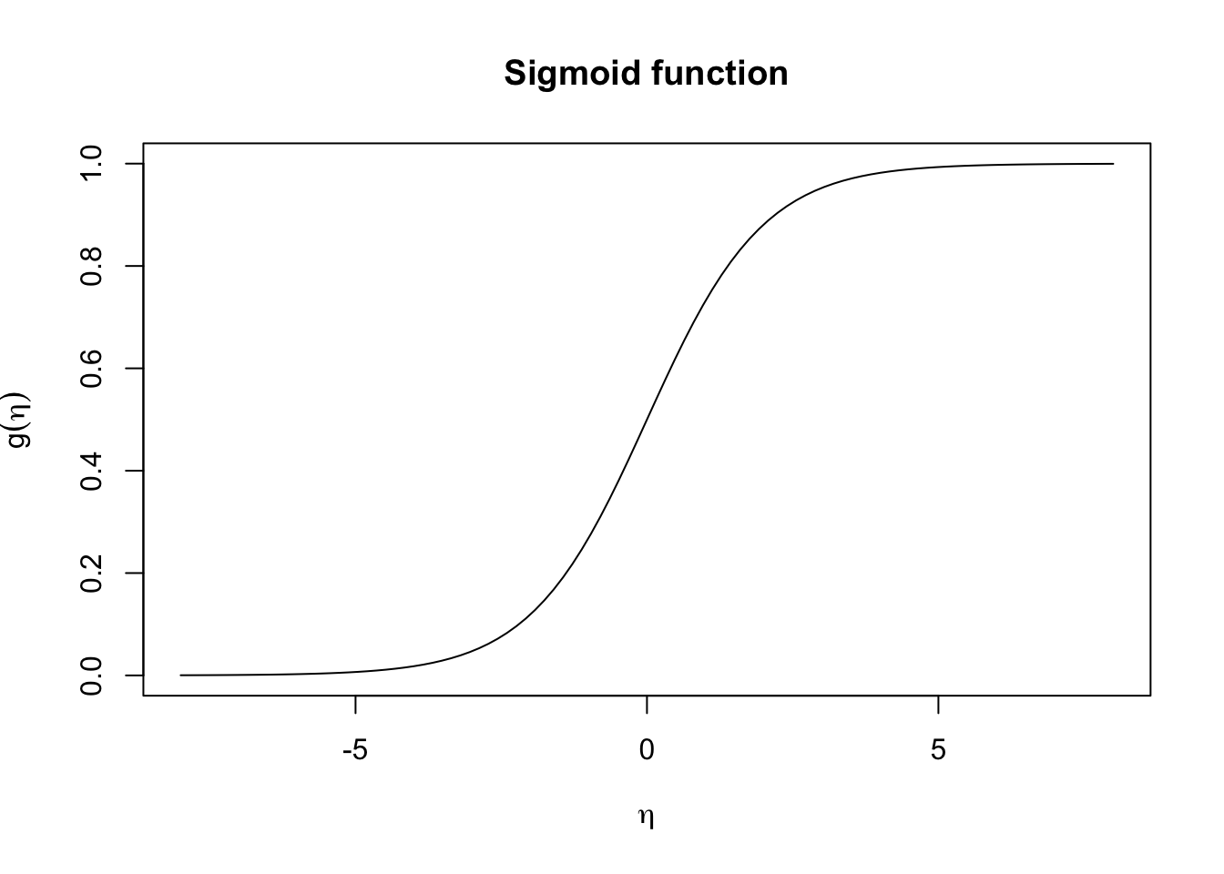
In logistic regression we use the logistic link function \(g(x) = \frac{1}{1 + e^{-x}}\) (i.e. sigmoid function) to map the linear combination of predictors, \(\eta\) to probabilities, where
\[\begin{align*} g(\eta) &= \Pr(Y = 1 \mid X = x) \\ &= \dfrac{1}{1 + e^{-\eta}}\\ &= \dfrac{1}{1+ e^{-(\beta_0 + \beta_1 X_1 + \cdots \beta_p X_p)}} \end{align*}\]
In other words, this will transforms the linear predictor \(\eta = \beta_0 + \beta_1 X_1 + \cdots \beta_p X_p\) into a value between 0 and 1.
Alternatively you can think of this in terms of \(g^{-1}()\), i.e., the inverse link function, which is the logit function, \(\text{logit}(p) = \ln \left( \frac{p}{1-p} \right)\) in the case of logistic regression.
\[ \begin{align*} g(\eta) &= \mu \\ \implies \eta &= g^{-1}(\mu) \\ &= \ln \left( \frac{\mu}{1-\mu} \right) \end{align*} \]
In other words, the linear predictor \(\eta = \beta_0 + \beta_1 x_1 + \cdots \beta_p x_p\) provides the log-odds of \(Y = 1\) given some particular set of \((x_1, x_2, \dots, x_p)\) values.
Logistic Regression:
\[ \text{log odds} = \beta_0 + \beta_1 X_1 + \dots + \beta_p X_p \]
Assumptions
\[ \begin{align} Y_i &\sim \text{Bernoulli}(\pi_i) = \mu \\ g( \eta) & = \dfrac{1}{1+e^{-\sum_{j=1}^p\beta_j X_j}} \end{align} \]
where \(g(\cdot)\) is the logistic function. Note: parameters are fit by maximum likelihood estimation (MLE) rather than ordinary least squares (OLS).
Interpretation of Coefficients
Since probability \(\pi_i\) is non-linear as \(X\) varies6, we cannot interpret the coefficients as we did in regular regression. The best we can do is talk about the direction:
Holding all other variables constant, if \(\beta_j\) is positive, then an increase in \(X_j\) is associated with an increase in \(\pi_i\)
Holding all other variables constant, if \(\beta_j\) is negative, then an increase in \(X_j\) is associated with a decrease in \(\pi_i\).
R code
You can fit a logistic regression using the glm() function.
glm(formula, family = gaussian, data, ...)| Arguments | Description |
|---|---|
formula |
a symbolic description of the model to be fitted, eg Y~ X1 + X2 |
family |
a description of the error distribution and link function to be used in the model ?family |
data |
data frame (usually your training set) |
To perform logistic regression with a binary outcome we need to set family = “binomial”. Other options (not be covered in this course) include:
family = "gaussian"same aslm()family = "poisson"for predicting countsfamily = multinomialfor \(>2\) classesfamily = binomial('probit')probit regression (a common alternative to logistic regression)
A note about factor levels
Note that logistics regression takes the second level of a factor to be the \(Y = 1\).
Example
Using a single predictor
library(gclus)
data(body)
attach(body)

body$Gender <- factor(Gender)

simlog <- glm(Gender ~ Height , family="binomial", data = body)

# store the beta hats for easy referencing
betas <- coef(simlog)

# plot the data (renaming the y-axis)
plot(Gender~Height, ylab="Probility of being Male")

# plot the fitted curve p(x) = e^(b0+b2x)/(1 + e^(b0+b2x))
curve(
  (exp(betas[1] + betas[2]*x))/(1+exp(betas[1] + betas[2]*x)),
  add=TRUE, # superimposes onto scatterplot (otherwise new plot)
  lwd=2, # line width (make the line a bit thicker)
col=2) # 2 = red 
On paper we can calculate the \(\Pr(Y = 1 \mid X = x)\) using the formula
\[\begin{align*} \Pr(Y = y \mid X = 175) &= \dfrac{1}{1+ e^{-(\beta_0 + \beta_1 X_1 )}}\\ &= \dfrac{1}{1+ e^{-(-46.7632791 + 0.2729192 (175))}}\\ &= 0.7305827 \end{align*}\]
In R we could obtain these predictions using the predict() function:
newpt = data.frame(Height = 175)
predict(simlog, newdata = newpt, type="response")
1
0.7305827 We can also find the Height value that gives the linear boundary between the two prediction regions.
\[ \begin{align} \Pr(Y = y \mid \texttt{Height} = x) &= \dfrac{1}{1+ e^{-(\beta_0 + \beta_1 X_1 )}}\\ 0.5 &= \dfrac{1}{1+ e^{-(\beta_0 + \beta_1 X_1 )}} \\ 1 &= 0.5 + 0.5 \times e^{-(\beta_0 + \beta_1 X_1 )}\\ \frac{0.5}{0.5} &= e^{-(\beta_0 + \beta_1 X_1 )}\\ \log \left(1\right) &= {\beta_0 + \beta_1 X} \\ \implies X &= -\frac{\beta_0}{\beta_1} \end{align} \] So for Height \(> -\dfrac{ -46.7632791}{0.2729192} = 171.34\) we would predict Male.
Using multiple predictors
# Fit the logistic regression model
mlr <- glm(factor(Gender) ~ Height + WaistG + BicepG, family="binomial")
summary(mlr)
Call:
glm(formula = factor(Gender) ~ Height + WaistG + BicepG, family = "binomial")

Coefficients:
             Estimate Std. Error z value Pr(>|z|)
(Intercept) -55.32670    5.51960 -10.024  < 2e-16 ***
Height        0.21534    0.02864   7.520 5.50e-14 ***
WaistG        0.05167    0.02891   1.787   0.0739 .
BicepG        0.46541    0.08265   5.631 1.79e-08 ***
---
Signif. codes:  0 '***' 0.001 '**' 0.01 '*' 0.05 '.' 0.1 ' ' 1

(Dispersion parameter for binomial family taken to be 1)

    Null deviance: 702.52  on 506  degrees of freedom
Residual deviance: 232.90  on 503  degrees of freedom
AIC: 240.9

Number of Fisher Scoring iterations: 6
In this case, larger predictor values would result in higher probabilities that the observation is male.
Similar extensions/discussion as said in linear regression. See Midterm 2 Review
Discriminant Analysis
Discriminant Analysis is a statistical technique used for classification tasks, where the goal is to assign observations to predefined groups (or classes) based on their features. It models the relationship between the predictor variables (features) and the categorical outcome variable (class labels) by estimating probabilities of class membership.
Linear Discriminant Analysis (LDA):
- Model: Assumes that the features are normally distributed and have a common covariance matrix for all classes. LDA seeks a linear combination of features that best separates multiple classes.
- Objective: Maximizes the between-class variance relative to the within-class variance.
- Use Cases: Effective when the classes have similar covariance matrices and features are normally distributed.
Quadratic Discriminant Analysis (QDA):
- Model: Relaxation of LDA, allowing each class to have its own covariance matrix. QDA models a quadratic decision boundary.
- Objective: Maximizes the likelihood of the observed data under the assumption of a quadratic decision boundary.
- Use Cases: Useful when the assumption of a common covariance matrix is not appropriate, and the decision boundaries between classes are quadratic.
Be sure to know:
- the assumptions of LDA vs. QDA (and when to use which)
- the derivation of linear boundary
Unsupervised Learning
Unsupervised learning is a type of machine learning that deals with data without predefined labels or outcomes. Unlike supervised learning, where models are trained on labeled data to predict outcomes, unsupervised learning algorithms aim to discover hidden patterns, structures, or relationships within the data itself. This approach is particularly useful for exploratory data analysis, anomaly detection, and when you lack labeled data.
Two primary methods in unsupervised learning are clustering and dimensionality reduction.
Distances
Clustering methods in machine learning are techniques that group similar data points into distinct clusters or groups based on certain criteria. These methods aim to discover hidden patterns or structures in the data without prior knowledge of the class labels. Distance play a crucial role many machine learning models. In this course we explored a few different types of distance calculations:
Euclidean Distance
The Euclidean distance between observations \(x_i = (x_{i1}, x_{i2}, \dots x_{ip})\) and \(x_j = (x_{j1}, x_{j2}, \dots x_{jp})\) is calculated as \[d^{\text{EUC}}_{ij} = \sqrt{\sum_{k=1}^p (x_{ik} - x_{jk})^2}\]
We often normalize (scale and center the data to have mean 0, variance 1) via \[z_{ik} = \frac{x_{ik}-\mu_k}{\sigma_k}\] then we can define standardized pairwise distances as \[d^{\text{STA}}_{ij} = \sqrt{\sum_{k=1}^p (z_{ik} - z_{jk})^2}\]
Manhattan Distance
Manhattan distance7 measures pairwise distance as though one could only travel along the axes \[d^{\text{MAN}}_{ij} = \sum_{k=1}^p |x_{ik} - x_{jk}|\]
Similarly, one might want to consider the standardized form \[d^{\text{MANs}}_{ij} = \sum_{k=1}^p |z_{ik} - z_{jk}|\]
Mahalanobis Distance
Mahalanobis distance takes into account the covariance structure of the data.
It is easiest defined in matrix form \[d^{\text{MAH}}_{ij} = \sqrt{(x_i - x_j)^T \boldsymbol{\Sigma}^{-1} (x_i - x_j)}\] where \(^T\) represents the transpose of a matrix and \(^{-1}\) denotes the inverse of matrix.
Matching Binary Distance
We can actually define another matching method that is equivalent to Manhattan/city-block,
\[d^{\text{MAT}}_{ij} = \text{\# of variables with opposite value}\]
Asymmetric Binary Distance
Asymmetric binary distance is a measure of dissimilarity between two binary vectors (vectors with elements of 0 or 1) where differences in the presence or absence of certain features are considered unequal. The example we saw in class disregards 0-0 matches.
\[d^{\text{ASY}}_{ij} = \frac{\text{\# of 0-1 or 1-0 pairs}}{\text{\# of 0-1, 1-0, or 1-1 pairs}}\]
Distance for Qualitative Variables
For categorical variables having \(>2\) levels, a common measure is essentially standardized matching once again. \[d^{\text{CAT}}_{ij} = 1 - \frac{u}{p}\]
where \(u\) is the number of variables that match between observations \(i\) and \(j\) and
\(p\) is the total number of variables
Gower’s Distance
Gower’s distance (or Gower’s dissimilarity) is calculated as: \[d^{\text{GOW}}_{ij} = \frac{\sum_{k=1}^p \delta_{ijk} d_{ijk}}{\sum_{k=1}^p \delta_{ijk}}\]
where
- \(\delta_{ijk}\) = 1 if both \(x_{ik}\) and \(x_{jk}\) are non-missing (0 otherwise),
- \(d_{ijk}\) depends on variable type
- Quantitative numeric \[d_{ijk} = \frac{|x_{ik} - x_{jk}|}{\text{range of variable k}}\]
- Qualitative (nominal, categorical) \[d_{ijk} = \begin{cases} 0 \text{ if obs i and j agree on variable k, } \\ 1 \text{ otherwise} \end{cases} \]
- Binary \(d_{ijk} = \begin{cases} 0 \text{ if obs i and j are a 1-1 match, } \\ 1 \text{ otherwise} \end{cases}\)
Clustering
Hierarchical clustering
As its name suggests, hierarchical clustering is a type of clustering algorithm that builds a hierarchy of clusters.
There are two main types of hierarchical clustering:
Agglomerative (bottom-up approach) Hierarchical Clustering: starts with each data point as a separate cluster and then iteratively merges the closest clusters until only one cluster remains.
Divisive (top-down) Hierarchical Clustering: starts with all data points in a single cluster and then recursively splits the cluster into smaller clusters until each data point is in its own individual cluster.
We focus on agglomerative hierarchical clustering which takes the following steps:
Initialization: Start by treating each data point as a separate cluster. At the beginning, there are as many clusters as there are data points.
Compute Similarities/Distances: Calculate the pairwise distances or similarities between all clusters. The choice of distance metric depends on the nature of the data (e.g., Euclidean distance, Manhattan distance, etc.).
Merge Closest Clusters: Identify the two closest clusters based on the computed distances or similarities. The definition of “closeness” depends on the chosen distance metric.
Update Cluster Set:: Merge the two closest clusters into a single cluster, reducing the total number of clusters by one.
Repeat steps 2–4: Recalculate the distances or similarities between the updated clusters and repeat the process of identifying and merging the closest clusters. For this we must choose a linkage criteria (how to measure the distance between clusters). Common linkage methods include:
- Single linkage: calculates the minimum distance between two points in each cluster.
- Complete linkage: calculates the maximum distance between two points in each cluster.
- Average linkage: calculates the average pairwise distance between the observations inside group with those outside.
- Centroid Linkage: calculates the distance between the centroids (mean points) of two clusters.
In some cases, the choice of linkage method could make a big difference. (e.g. single linkage often leads to “chaining” which produces elongated clusters.
- Termination: Continue this process iteratively until only one cluster, containing all the data points, remains.
Don’t forget to normalize your data (we use the scale(x, center = TRUE, scale = TRUE) function for that)!
Dendrogram Construction:
Throughout the process, keep track of the merging order and heights at which merges occur. This information is used to construct a dendrogram, which visually represents the hierarchy of clusters.
data(faithful)
colors <- c("purple",
 "dodgerblue",
 "firebrick",
 "forestgreen",
 "gold")
fait <- hclust(dist(scale(faithful)), method="single")
plot(fait, main="", labels=FALSE)
hc2 <- cutree(fait, k = 2)
plot(faithful, col = colors[hc2], pch=as.character(hc2))
- Dendrograms can also be used to determine how many groups are present in the data.
- The number of clusters is determined by cutting the dendrogram at a certain height
- Generally, we can “cut” at the largest jump in distance, and that will determine the number of groups, as well as each observation’s group membership.
kmeans clustering
\(k\)-means clustering is a popular method for grouping n observations into \(k\) clusters; note that \(k\) needs to be provided by the user.
Method: Divides the dataset into k clusters by assigning data points to the cluster whose centroid (mean) is closest to them.
Objective: Minimizes the within-cluster sum of squares.
Use Cases: Effective for spherical clusters with similar sizes.
Algorithm
- Randomly select \(k\) (the number of groups) points in your data. These will serve as the first centroids8
- Assign all observations to their closest centroid (in terms of Euclidean distance). You now have \(k\) groups.
- Calculate the means of observations from each group; these are your new centroids.
- Repeat 2) and 3) until nothing changes anymore (each loop is called an iteration).
Objective: to minimize Within-Cluster-Sum of Squared Errors (WSS) , i.e. the sum of squared distances between the points and their respective cluster centroid.
Note that this alogrithm is stochastic (you may get a different answer based the random assignment in step 1.) To gain some stability we will often run the algorithm several times and pick the best one (in terms of WSS). For example, we can run kmeans 25 times using:
kmeans(x, centers=k, nstart = 25)Elbow method
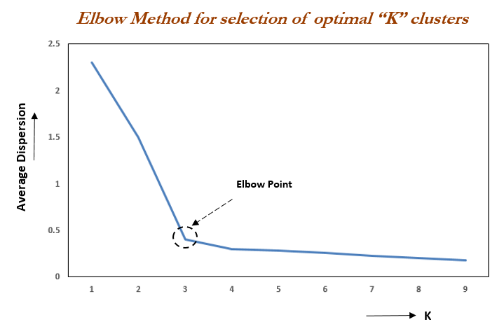
To choose the value of \(k\) we can use the “elbow method”. It works as follows:
- Calculate the Within-Cluster-Sum of Squared Errors (WSS) for different values of \(k\),
- Choose the \(k\) for which WSS becomes first starts to diminish.
This appears int the WSS-versus-\(k\) plot (aka scree plot) in the form of an “elbow”.
Gaussian Mixture Models (GMM):
- Method: Models data as a mixture of several Gaussian distributions, allowing for flexibility in cluster shapes.
- Objective: Maximizes the likelihood of the observed data under the assumption of a Gaussian mixture.
- Use Cases: Applicable when clusters have different shapes and are not necessarily spherical.
K-means and hierarchical clustering relies on Euclidean distances. We also looked at other distance measures, including: Manhattan, Mahalanobis, Matching Binary, Asymmetric Binary, and Gower’s Distance.
- know the basic differences between these, and when you can use them (e.g. which can be used with categorical predictors).
Dimensionality Reduction
Reduces the number of features or variables in the dataset while preserving relevant information. This is particularly useful for visualizing high-dimensional data and improving computational efficiency. The method we looked at for achieving this was PCA (there are others)
Principal Component Analysis (PCA)
Principal Component Analysis (PCA) is a dimensionality reduction technique widely used in machine learning and data analysis. It aims to transform a dataset with potentially correlated features into a new set of uncorrelated features, called principal components, that capture the maximum variance in the data. PCA is particularly useful for visualizing high-dimensional data, reducing computational complexity, and identifying important patterns.
Steps in PCA:
Standardize the features to have zero mean and unit variance. This ensures that all features contribute equally to the covariance matrix.
Compute Covariance Matrix from the standardized data. The covariance matrix represents the relationships between different features, indicating how they vary together.
Perform Eigenvalue Decomposition on the covariance matrix to obtain eigenvectors and eigenvalues.
Eigenvectors: Represent the directions of maximum variance in the data.
Eigenvalues: Indicate the magnitude of variance along the corresponding eigenvector.
Interpret the Principal Components:
Principal components are the eigenvectors obtained from the eigenvalue decomposition. They form a new set of orthogonal axes that capture the most significant variability in the data.
The first principal component corresponds to the direction of maximum variance, the second to the second-highest variance, and so on, …
Select Principal Components: Choose a subset of the eigenvectors (principal components) based on the desired amount of retained variance, or the Kaiser criterion, or the elbow method.
Transform Data: Project the original data onto the selected principal components to obtain the reduced-dimensional representation. If the number of components \(M\) is less than the original number of predictors in the data \(p\), this results in a transformed dataset with reduced dimensionality (otherwise it represents a rotation of the data).
Use Cases:
Dimensionality Reduction:
- PCA is often used to reduce the number of features in a dataset while retaining most of the variability.
Visualization:
- Visualizing high-dimensional data in a lower-dimensional space is a common application of PCA, especially in scatter plots.
Noise Reduction:
- By focusing on the principal components with the highest variance, PCA can help reduce the impact of noise in the data.
Feature Engineering:
- PCA-derived features can be used as input for downstream machine learning models.
Identifying Important Features:
- The contribution of each original feature to principal components provides insights into the importance of different features.
Know how to:
pick the number of appropriate PCs (e.g. prop of variance explained, read an elbow-plot, kaiser criterion)
Assess what a principal component represents
interpret a bi-plot
Footnotes
\(B\) is usually quite is large (1000, 5000 are standard amounts)↩︎
where \(n\) is equal to the number of samples in your original data set↩︎
AKA city-block distance, L1 distance, \(\ell_1\) norm, or Taxicab geometry↩︎
where one class has significantly more instances than the other class or classes.↩︎
independent variable is a perfect linear function of other explanatory variables↩︎
in logistic regression, increasing \(X\) by one unit changes the log odds by \(\beta_1\)↩︎
AKA city-block distance, L1 distance, \(\ell_1\) norm, or Taxicab geometry↩︎
\(B\) is usually quite is large (1000, 5000 are standard amounts)↩︎