Type I/II Errors and Power

STAT 205: Introduction to Mathematical Statistics

Dr. Irene Vrbik

University of British Columbia Okanagan

Review

In Hypothesis Testing, we begin with a null hypothesis, which generally asserts that there is no effect between our treatment and control groups. Commonly, this is expressed as the difference in means between the treatment and control groups being zero.

\[\begin{align} H_0: \theta = \theta_0 \quad\quad \text{ vs } \quad\quad H_A: \begin{cases} \theta < \theta_0\\ \theta > \theta_0\\ \theta \neq \theta_0 \end{cases} \end{align}\]

Population

👩‍⚕️👨‍🍳🧑‍🔬👩‍🎨👨‍🚀🧑‍🏫👩‍✈️👨‍⚖️🧑‍🌾👩‍🔧👨‍🎤🧑‍🏭👩‍🚒👨‍🎓🧑‍⚕️👩‍🔬👨‍🎨🧑‍🚀👩‍🏭👨‍🔧

\(\downarrow\)

Sample

👨‍🚀 👩‍✈️ 👩‍🔬 🧑‍🌾 🧑‍🚀

Review

Sample

👨‍🚀 👩‍✈️ 👩‍🔬 🧑‍🌾 🧑‍🚀

\(\downarrow\)

\[ \hat \theta \]

\(\downarrow\)

from this sample statistic we derive a sampling distribution

we define a test statistic that follows some common distriubtion

Null Distribution

these are examples of possible realizations of our test statistic

some will fall in the acceptance region leading us to the decision not to reject the null

some will fall in the rejection region and lead us to reject H₀

Important there will be instances when the null hypothesis is true and we reject it. This is called a Type I error

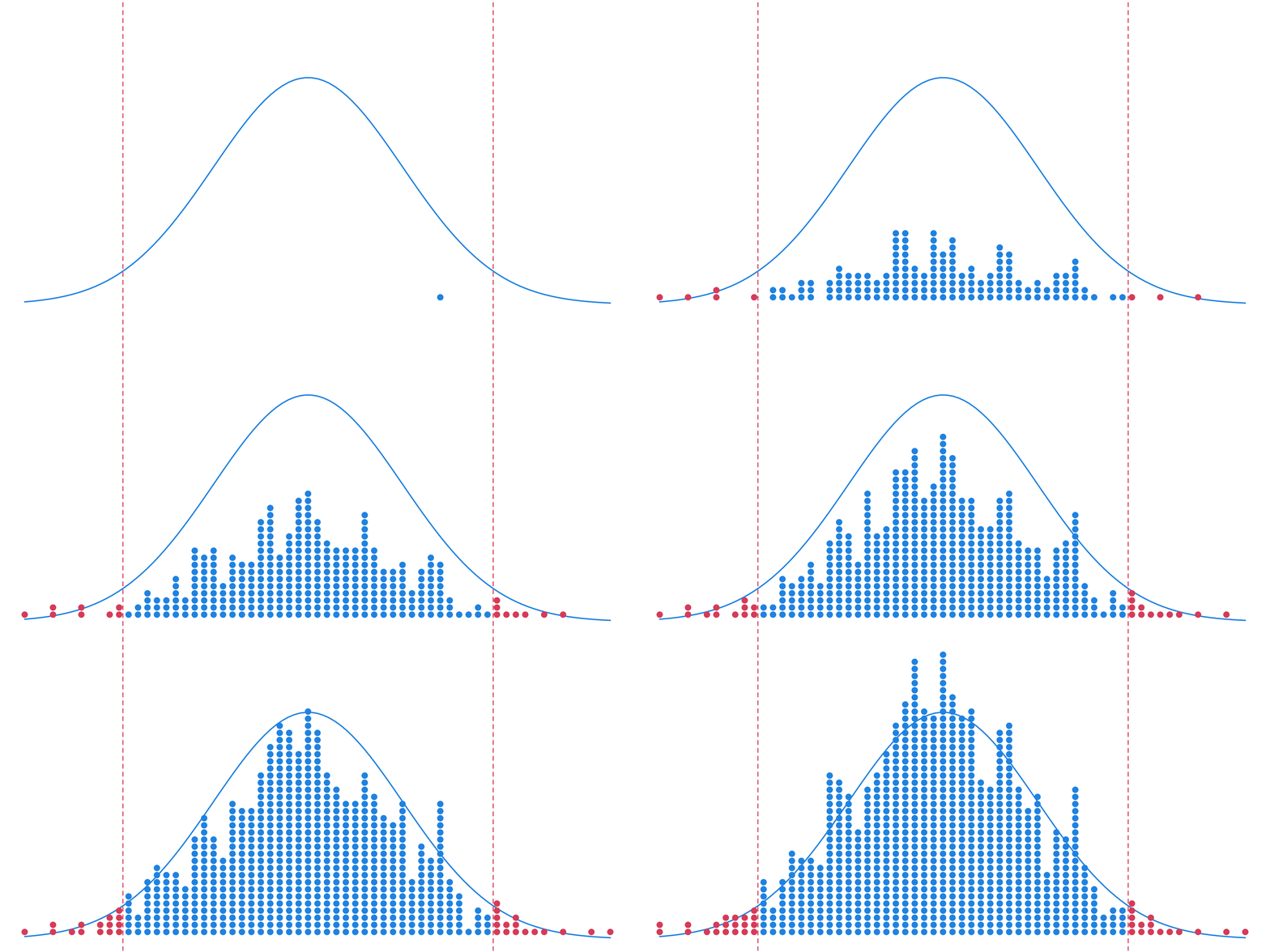
Coin Flip Example

We want to investigate whether or not a coin is fair¹

\[ \begin{align} H_0: &p = 0.5 && H_A: &p \neq 0.5 \end{align} \]

• To test this hypothesis, let’s generate some samples under the null hypothesis.

• In other words, let’s flip a fair coin 30 times, count the number of heads, and check for significance.

if the coin in fair we would expect 50% of the tosses to be H/T if we tossed the coin an infinite amount of times

or course in a finite sample, if the coin is fair we would expect roughly 50% of the tosses to land H/T but we know this experiment is subject to randomness

Note: Since \(np_0 = n(1-p_0)= 30*0.5 = 15 > 10\) we can trust that the sampling distribution of \(\hat p\) is approximately normal.

1. i.e. 50% of the time it lands “Heads” , 50% of the time it lands “Tails”

Simulation 1

Rather than physically doing this with a coin, we can simulate coin flips using rbinom()¹

#   n = number or simulations 
#   size = trial size (number of coin flips)
#   prob =  probability getting heads on a given flip
set.seed(205)
num_heads <- rbinom(n = 1, size = 30, prob = 0.5)

[1] 21

Heads	Tails
21	9

\[\hat p = \dfrac{21}{30} = 0.7\]

1. run ?rbinom in the R Console for more details

Test Statistic

indeed that high frequency of heads in this sample lead us to reject the null hypothesis that the coin is fair

\[ \begin{align} Z &= \frac{\hat p - p_0}{\sqrt{\frac{p_0(1-p_0)}{n}}} \\ &=\frac{0.7 - 0.5}{\sqrt{\frac{0.5(1-0.5)}{30}}}\\ z_{obs}&= 2.191 \end{align} \]

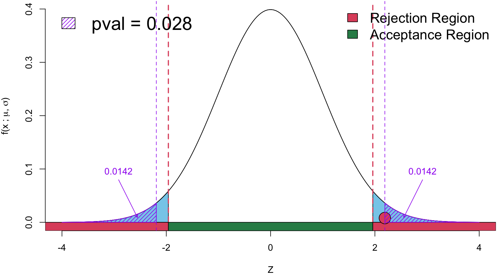
Conclusion Since the \(p\)-value is < \(\alpha\), there is sufficient statistical evidence to suggest that the the coin is fair.

but we KNOW the coin is fair, (we simulated with p = 0.5)

so what happened here is that we made a mistake (as indicated with a red dot)

Simulation 2

# Heads = 12 # Tails = 18

\[ \begin{align} Z &= \frac{\hat p - p_0}{\sqrt{\frac{p_0(1-p_0)}{n}}} \\ &=\frac{0.4 - 0.5}{\sqrt{\frac{0.5(1-0.5)}{30}}}\\ z_{obs}&= -1.095 \end{align} \]

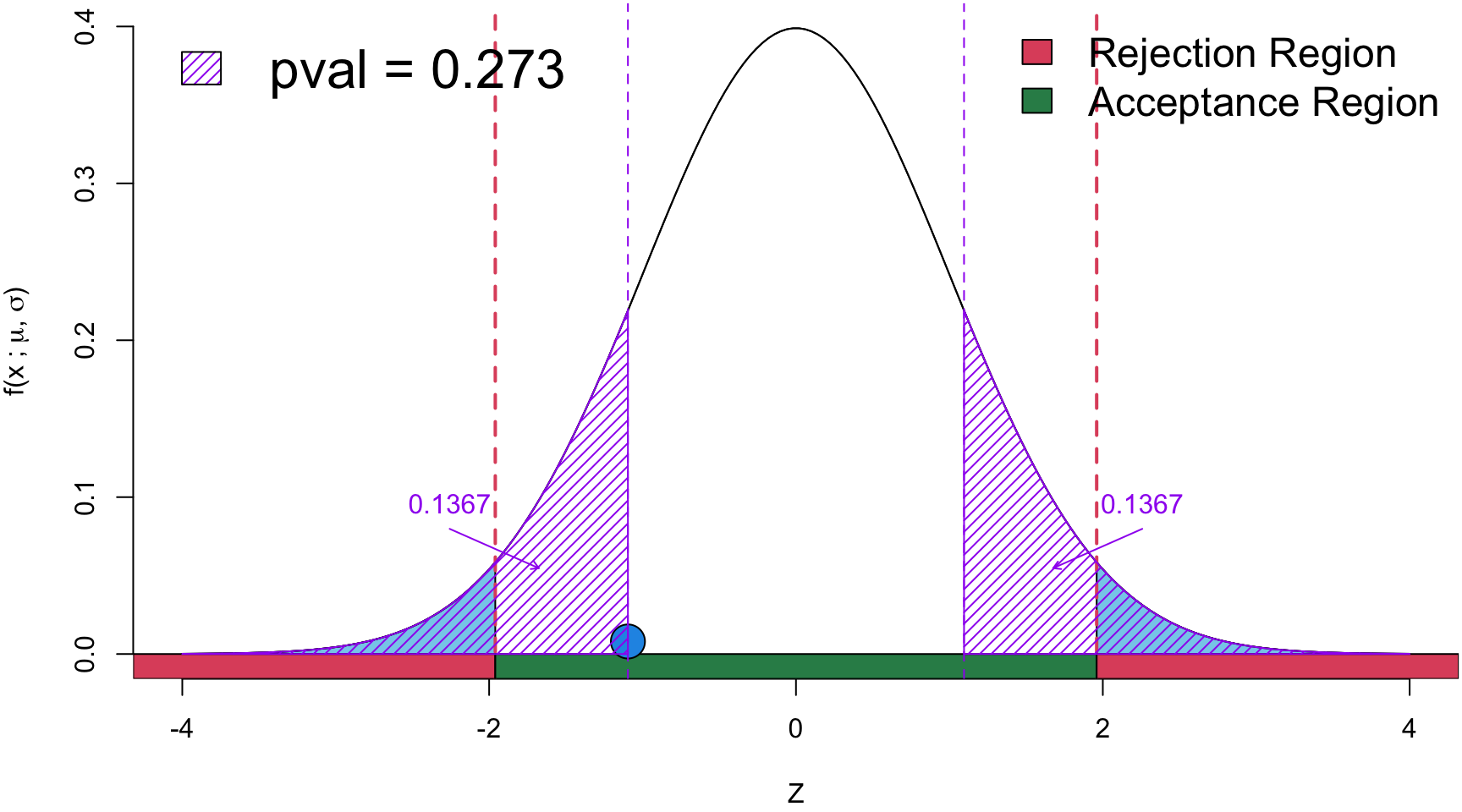
Conclusion Since the \(p\)-value is > \(\alpha\), there is insufficient statistical evidence to suggest that the the coin is fair.

Our estimate (see the test statistic calc) is different than our hypothesized value of 0.5

but as our p-value suggests its not statisticially significantly different

Simulation 3

# Heads = 15 # Tails = 15

\[ \begin{align} Z &= \frac{\hat p - p_0}{\sqrt{\frac{p_0(1-p_0)}{n}}} \\ &=\frac{0.5 - 0.5}{\sqrt{\frac{0.5(1-0.5)}{30}}}\\ z_{obs}&= 0 \end{align} \]

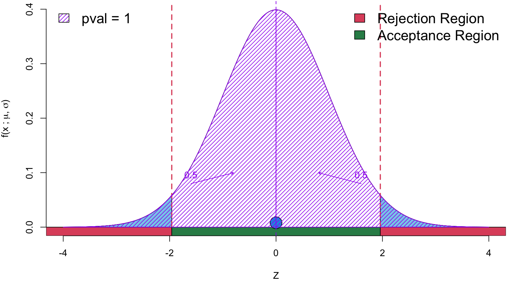
Conclusion Since the \(p\)-value is > \(\alpha\), there is insufficient statistical evidence to suggest that the the coin is fair.

Simulation4

# Heads = 17 # Tails = 13

\[ \begin{align} Z &= \frac{\hat p - p_0}{\sqrt{\frac{p_0(1-p_0)}{n}}} \\ &=\frac{0.57 - 0.5}{\sqrt{\frac{0.5(1-0.5)}{30}}}\\ z_{obs}&= 0.73 \end{align} \]

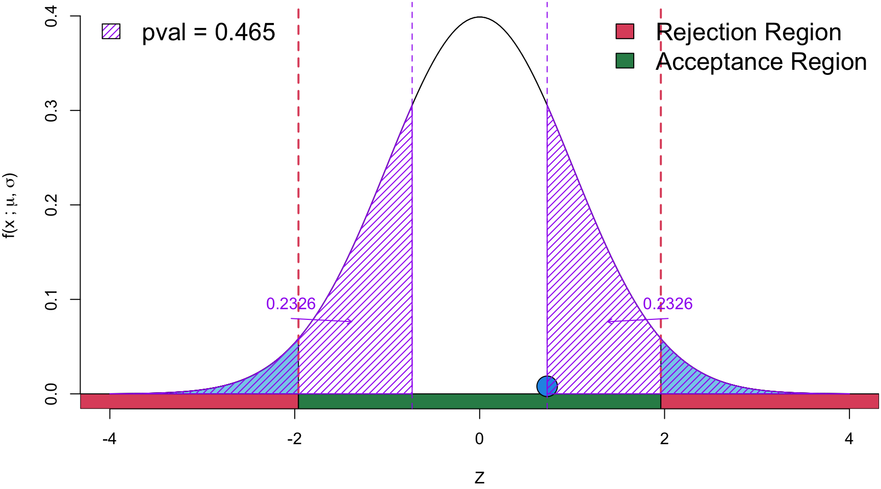
Conclusion Since the \(p\)-value is > \(\alpha\), there is insufficient statistical evidence to suggest that the the coin is fair.

Statistic 5

# Heads = 16 # Tails = 14

\[ \begin{align} Z &= \frac{\hat p - p_0}{\sqrt{\frac{p_0(1-p_0)}{n}}} \\ &=\frac{0.53 - 0.5}{\sqrt{\frac{0.5(1-0.5)}{30}}}\\ z_{obs}&= 0.365 \end{align} \]

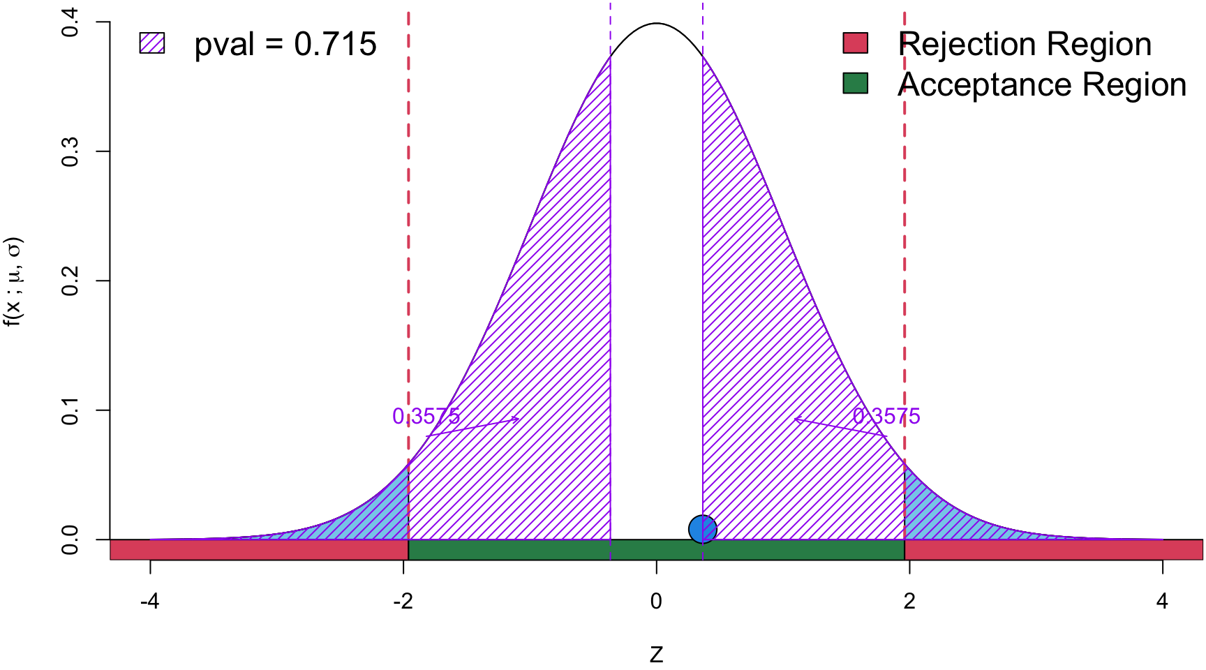
Conclusion Since the \(p\)-value is > \(\alpha\), there is insufficient statistical evidence to suggest that the the coin is fair.

Statistic 6

# Heads = 14 # Tails = 16

\[ \begin{align} Z &= \frac{\hat p - p_0}{\sqrt{\frac{p_0(1-p_0)}{n}}} \\ &=\frac{0.47 - 0.5}{\sqrt{\frac{0.5(1-0.5)}{30}}}\\ z_{obs}&= -0.365 \end{align} \]

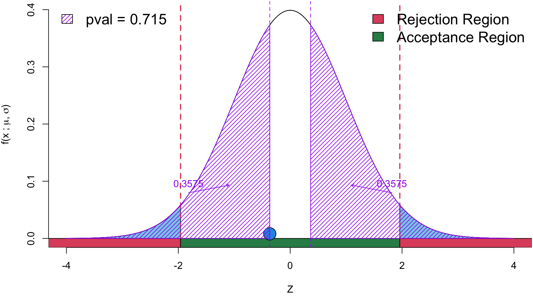
Conclusion Since the \(p\)-value is > \(\alpha\), there is insufficient statistical evidence to suggest that the the coin is fair.

Even if the null hypothesis is TRUE we are going to incorrectly reject it sometimes

iClicker

Unluckly Trails

If we repeat a simulation 100 times—where we flip a fair coin 30 times, count the number of heads, and perform a hypothesis test for fairness each time—how often would we expect to obtain a statistically significant¹ result? In other words, how many times would we expect to incorrectly reject \(H_0\) (the coin is fair) purely due to random chance?

1. 1-2 times
2. 5 times
3. 10 or more

4. 20 or more
5. I don’t know (you’ll get the mark for this too)

1. i.e. obtain a \(p\)-value < \(\alpha\)

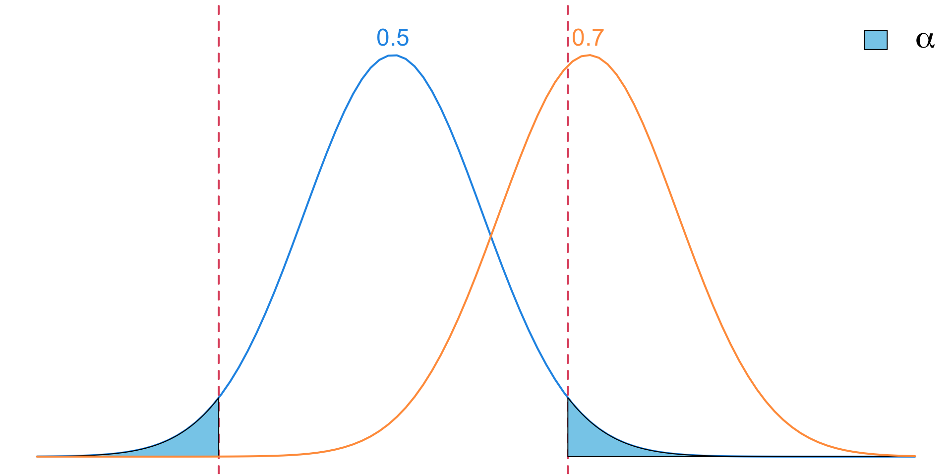
Type I Error

• A Type I Error occurs when we incorrectly reject the null hypothesis (\(H_0\)) even though it is actually TRUE.

• The probability of making a Type I error is \(\alpha\), i.e. the significance level.

• At this point you might be asking, why don’t we just set our significance level to 1%

• Well there is a tradeoff with another type of error,…

In any experiment, some random samples will show extreme values by chance, leading to false positives.

Decision Matrix

Reality

	\(H_0\) True	\(H_0\) False
Reject \(H_0\)	\(\textcolor{red}{\textsf{Type I error}}\)	\(\textcolor{green}{\textsf{Correct}}\)
Fail to reject \(H_0\)	\(\textcolor{green}{\textsf{Correct}}\)	\(\textcolor{red}{\textsf{Type II error}}\)

Here columns represent the reality or underlying true (that we never know), and rows represent out decision we make base on the hypothesis test.

column represent the reality, and rows represent out decision

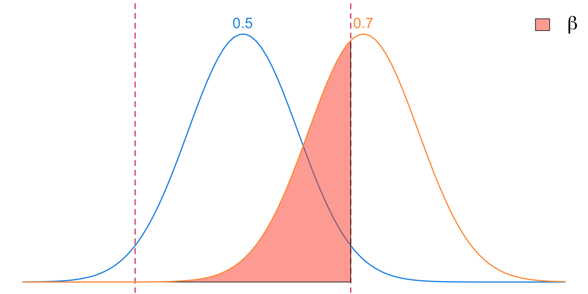
Type II Errors

• A Type II Error occurs when we incorrectly fail to reject the null hypothesis (\(H_0\)) even though it is actually FALSE.
• We denote the probability of making a Type II error by \(\beta\).
• As we will see, if we lower \(\alpha\) there will be less chance of Type I errors but an increases risk of Type II errors.
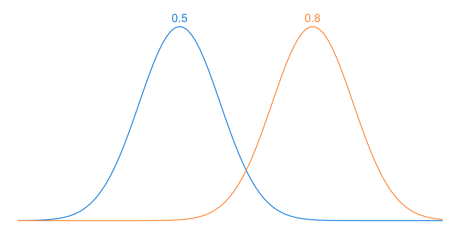
• Visualizing this one is a little harder since there are infinitely many alternative hypotheses for a given null hypothesis

we just choose one. None of them are more special or “real” than the others. 

Possibility 1

Possibility 2

Possibility 3

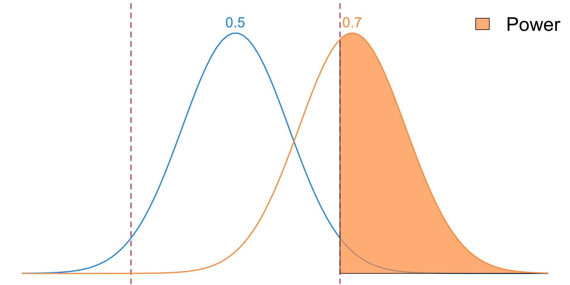
Power

\[ \begin{align} \text{Power} &= \Pr(\text{rejecting }H_0\mid H_0 \text{ false})\\ &= 1 - \Pr(\text{rejecting }H_0\mid H_0 \text{ false})\\ &= 1 - \Pr(\text{Type II error}\mid H_0 \text{ false})\\ &= 1 - \beta \\ &= \Pr(\text{not making a Type II error}\mid H_0 \text{ false}) \end{align} \]

Visualization of Type I

Visualization of Type II

Visualization of Power

Visualization Combined

iClicker: Identifying a Type I Error

Exercise 1 A university administrator is investigating whether the average GPA of students at her university is different from the national average of 3.2. She collects a random sample of students and performs a hypothesis test. Let \(\mu\) represent the true average GPA of students at her university and

\[ H_0: \mu = 3.2 \quad\quad H_a: \mu \neq 3.2 \]

Under which condition would the administrator commit a Type I error?

1. She concludes the university’s average GPA is not 3.2 when it actually is.

2. She concludes the university’s average GPA is not 3.2 when it actually is not.

3. She concludes the university’s average GPA is 3.2 when it actually is.

4. She concludes the university’s average GPA is 3.2 when it actually is not.

iClicker: Consequences of a Type II Error

Exercise 2 A company is evaluating whether to launch a new employee wellness program. They plan to survey a sample of employees to determine if more than 60% of them would be interested in participating. If there is strong evidence that interest exceeds 60%, they will proceed with implementing the program. Let \(p\) represent the proportion of employees interested in the wellness program and

\[ H_0: p = 0.60 \quad\quad H_a: p > 0.60 \]

What would be the consequence of a Type II error in this context?

1. They do not launch the wellness program when they should.

2. They do not launch the wellness program when they should not.

3. They launch the wellness program when they should not.

4. They launch the wellness program when they should.

Why is Power Important?

• A test with low power means we might not detect a real effect, leading to Type II errors.

• A high-power test increases the likelihood of detecting true differences.

• So how can we increase the power?

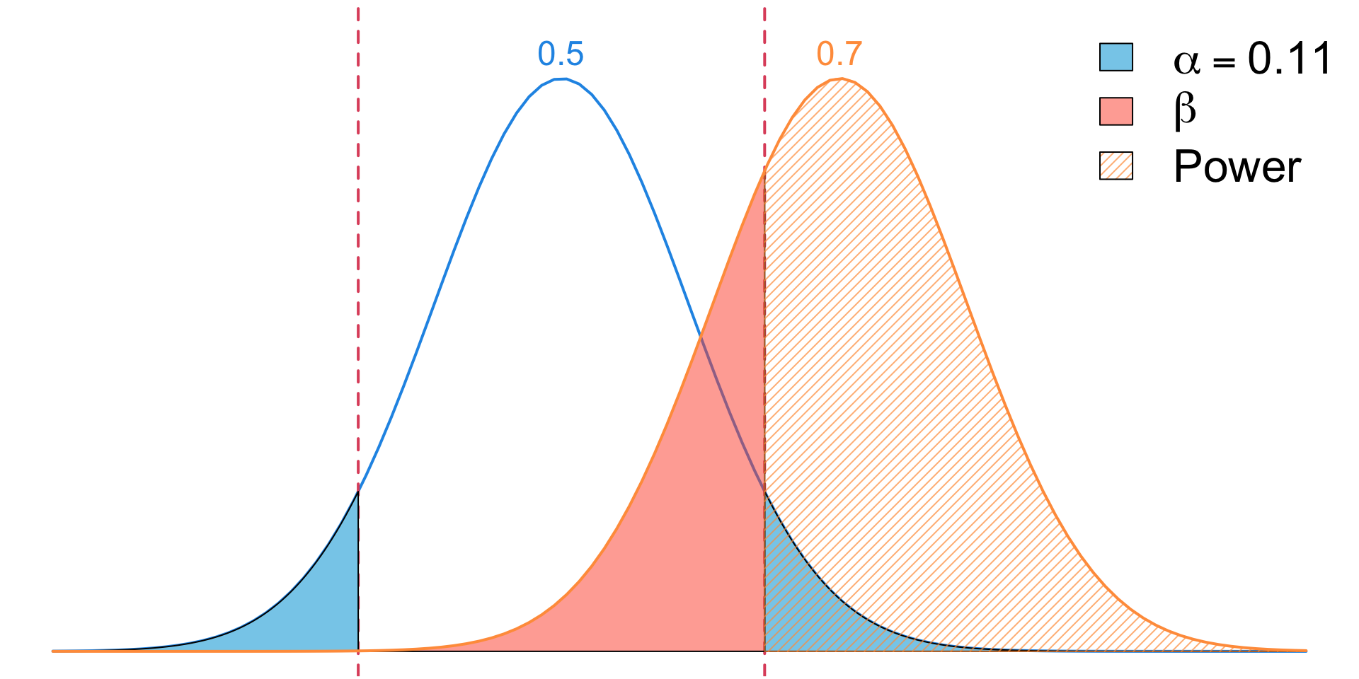
Increase Significance Level

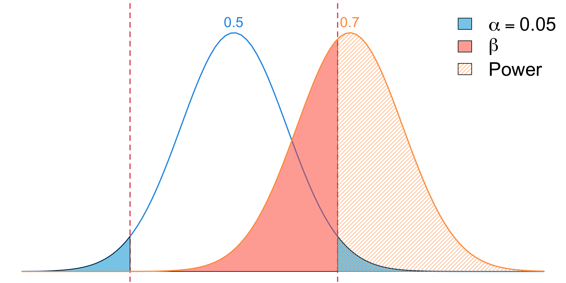
Increase Significance Level

As we increase the power, it comes at the cost of increase the probability of a Type I error

Depending on the type of analysis we might be willing to make that sacrifice, but it’s pretty standard to keep \(\alpha\) at 5% or 1%

Influences on Power

1. Significance Level (\(\alpha\))
   • Higher \(\alpha\) \(\implies\) Higher power
   • However, this also increases Type I errors

Increase Sample Size

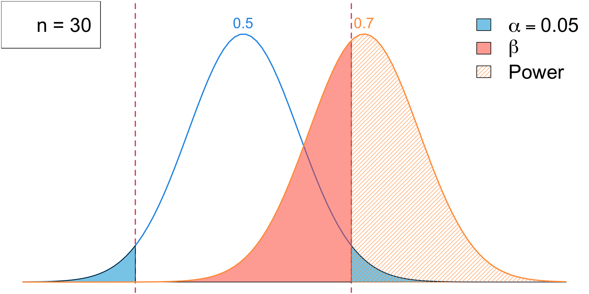
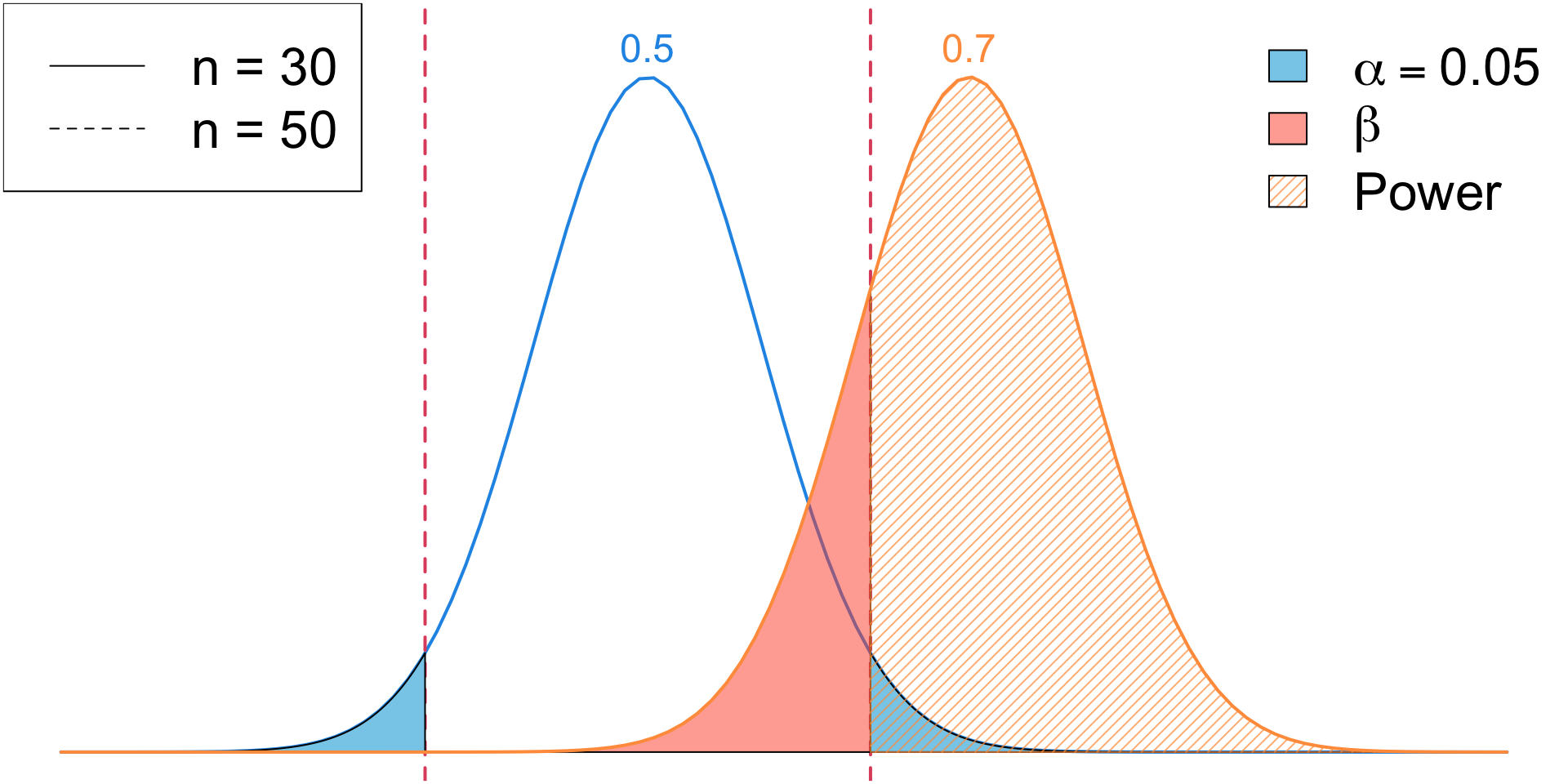
Increase Sample Size

Influences on Power

1. Significance Level (\(\alpha\))

   • Higher \(\alpha\) \(\implies\) Higher power
   • However, this also increases Type I errors

2. Sample Size (\(n\))

   • Increasing the sample size reduces variability, making it easier to detect small effects.
   • A test with \(n = 20\) might fail to detect a difference, while \(n=2000\) increases power significantly.

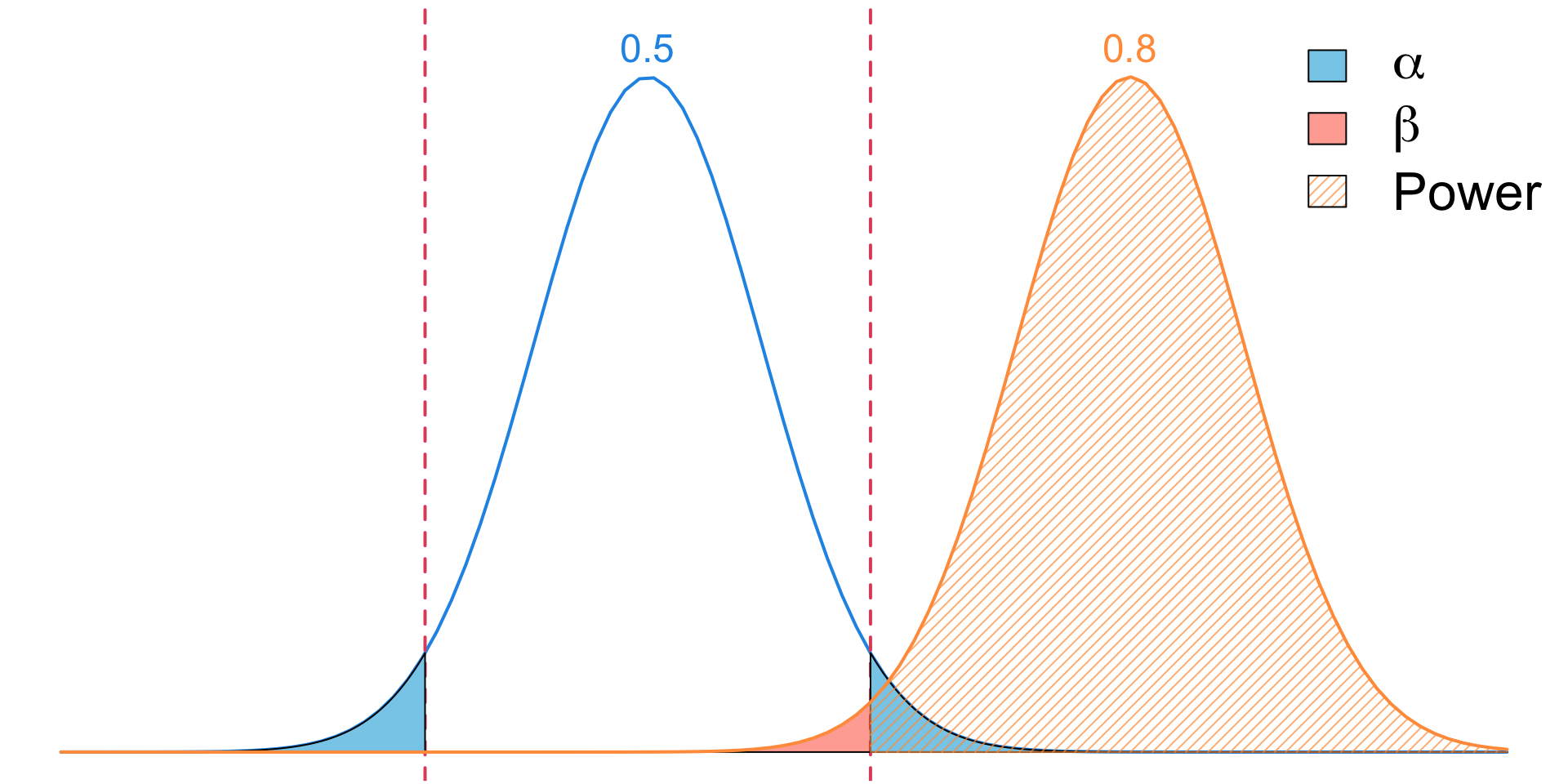
Increase Effect Size

Increase Effect Size

Effect Size

• In hypothesis tests for proportions, effect size refers to how different the true proportion (\(p\)) is from the null hypothesized proportion (\(p_0\)).

• Larger effect sizes make it easier to detect a difference, while smaller effect sizes require larger sample sizes for detection.

• For two sample tests for \(\mu\), the effect size (often denoted by \(\delta\)) is the magnitude of the difference between group means.

Influences on Power

1. Significance Level (\(\alpha\))

   • Higher \(\alpha\) \(\implies\) higher power
   • However, this also increases Type I errors

2. Sample Size (\(n\))

   • Increasing the sample size reduces variability, making it easier to detect small effects.

3. Effect Size (\(\delta\))

   • The larger the effect size, the higher the power

Definition

Type I Error (False Positive)

A Type I Error occurs when we incorrectly reject the null hypothesis (\(H_0\)) even though it is actually true. \(\Pr(\text{Type I error} \mid H_0 \text{ true}) = \alpha\).

Type II Error (False Negative)

A Type II Error occurs when we fail to reject the null hypothesis (\(H_0\)) even though the alternative hypothesis (\(H_A\)) is actually true. \(\Pr(\text{Type II error} \mid H_A \text{ true}) = \beta\).

Power (\(1- \beta\))

The power of a test is the probability of correctly rejecting (\(H_0\)) when \(H_A\)) is true. It measures the sensitivity of a test to detect an effect when one truly exists.

H_A true vs H₀

both arelogically equivalent, but the first one is clearer and more commonly used in statistical terminology

H₀ being false means that H_A is true by definition.

iClicker: Power

Identifying Statistical Power

Exercise 3 In the decision matrix shown below, which cell represents statistical power?

Reality	\(H_0\) True	\(H_0\) False
Reject \(H_0\)	(a) Type I error	(b) Correct
Fail to reject \(H_0\)	(c) Correct	(d) Type II error

(e) None of the above

Probability of a Type II Error and Power of a Test

Exercise 4 Suppose we are sampling 40 observations from a normally distributed population where it is known that the population standard deviation is \(\sigma = 8\), but the population mean \(\mu\) is unknown. We wish to test the hypotheses at a significance level of \(\alpha = 0.05\).

\[ H_0: \mu = 100 \quad \quad H_1: \mu < 100 \]

Suppose, in reality, the null hypothesis is false, and the true mean is \(\mu = 98\).

1. What is the probability of making a Type II error?
   
2. What is the power of the test?

Step 1: Determine the Critical Value

The rejection region under the null is:

Critical Z-Value

We can express the rejection region on terms of \(\bar X \sim N(100, 8/\sqrt{40})\)

Critical Value in terms of \(\bar X\)

The critical value for \(\bar{X}\) is determined by:

\[ P\left( \bar{X} < x_{\text{crit}} \mid H_0 \text{ true} \right) = \alpha \]

Since \(\bar{X} \sim N\left( 100, \frac{8}{\sqrt{40}} \right) = N(100, 1.265)\) we know

\[ Z = \frac{X - 100}{1.265} \sim N(0, 1) \] So we can reverse transform \[ z^* = \frac{x_{\text{crit}} - 100}{1.265} \]

where \(z^* = -1.645\) is the critical \(z\)-score. Solving for \(x_{\text{crit}}\):

\[ x_{\text{crit}} = 100 + (-1.645)(1.265) = 97.92 \]

Step 2: Probability of Type II Error (\(\beta\))

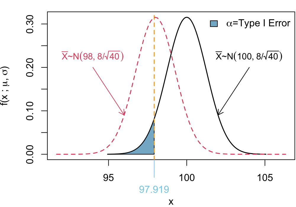
Type II Error set up

A Type II error occurs when \(H_0\) is false (\(\mu = 98\)), but we fail to reject it. That happens when:

\[ P\left( \bar{X} > 97.92 \mid H_a: \mu = 98 \right) \]

Under \(H_a\), the distribution of \(\bar{X}\) is:

\[ \bar{X} \sim N(98, 1.265) \]

Finding the corresponding \(Z\)-score:

\[ Z = \frac{97.92 - 98}{1.265} = \frac{-0.08}{1.265} = -0.063 \]

From the standard normal table:

\[ \begin{align} P(Z > -0.063) &= 1 - P(Z < -0.063) \\ &= 1 - 0.475 = 0.525 \end{align} \]

Thus, the probability of a Type II error is:

\[ \beta = 0.525 \]

Illustration of Type II Error

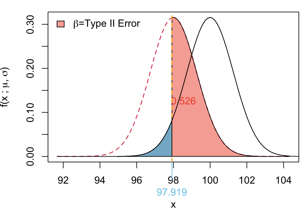
Type II Error

Step 3: Compute the Power of the Test

The power of the test is:

\[ \text{Power} = 1 - \beta = 1 - 0.525 = 0.475 \]

This means the test has a 47.5% chance of correctly rejecting \(H_0\) when \(\mu = 98\).

Illustration of Power

Power of the Test

Detecting Defective Light Bulbs

Exercise 5 A light bulb manufacturer claims that the mean lifetime of its energy-saving bulbs is 800 hours. A consumer advocacy group suspects that the true mean lifetime is actually less than 800 hours and decides to test the claim.

A random sample of 50 light bulbs is selected, and their lifetimes are measured. It is known that the population standard deviation of light bulb lifetimes is 30 hours. The consumer group sets up the following hypothesis test at \(\alpha = 0.05\):

\[ H_0: \mu = 800 \quad \quad H_a: \mu < 800 \]

Suppose in reality, the true mean lifetime is 790 hours.

1. What is the probability of making a Type II error?
   
2. What is the power of the test?

Step 1: Determine the critical value

The test is one-sided (left-tailed), and we reject \(H_0\) if the sample mean \(\bar{X}\) is sufficiently low. The critical value for \(\bar{X}\) is determined by:

\[ P\left( \bar{X} < x_{\text{crit}} \mid H_0 \text{ true} \right) = \alpha \]

Since \(\bar{X}\) follows a normal distribution:

\[ \bar{X} \sim N\left( \mu_0, \frac{\sigma}{\sqrt{n}} \right) \]

Substituting known values:

\[ \bar{X} \sim N\left( 800, \frac{30}{\sqrt{50}} \right) = N(800, 4.24) \]

Using \(Z\)-scores:

\[ Z = \frac{x_{\text{crit}} - 800}{4.24} \]

From standard normal tables, for \(\alpha = 0.05\), the critical \(Z\)-score is:

\[ Z_{\alpha} = -1.645 \]

Solving for \(x_{\text{crit}}\):

\[ x_{\text{crit}} = 800 + (-1.645)(4.24) = 793.03 \]

Step 2: Find \(\beta\) (Probability of Type II Error)

A Type II error occurs when \(H_0\) is false (i.e., \(\mu = 790\)), but we fail to reject it. That happens when:

\[ P\left( \bar{X} > 793.03 \mid H_a: \mu = 790 \right) \]

Under \(H_a\), the distribution of \(\bar{X}\) is:

\[ \bar{X} \sim N(790, 4.24) \]

Finding the corresponding \(Z\)-score:

\[ Z = \frac{793.03 - 790}{4.24} = \frac{3.03}{4.24} = 0.715 \]

From standard normal tables:

\[ P(Z > 0.715) = 1 - P(Z < 0.715) = 1 - 0.762 = 0.238 \]

Thus, the probability of a Type II error is:

\[ \beta = 0.238 \]

Step 3: Compute the Power of the Test

The power of the test is:

\[ \text{Power} = 1 - \beta = 1 - 0.238 = 0.762 \]

Resources

• https://www.statsig.com/blog/hypothesis-testing-explained
• https://statisticsbyjim.com/hypothesis-testing/types-errors-hypothesis-testing/