Examples with t-test

STAT 205: Introduction to Mathematical Statistics

Dr. Irene Vrbik

University of British Columbia Okanagan

Lecture Learning outcomes

By the end of this lecture students should be able to complete “by hand” and using the t.test() function.

1. Paired \(t\)-test for dependent groups
2. Pooled \(t\)-test for independent groups with equal variance
3. Welch’s procedure (approximate \(t\)-test) for independent groups with unequal variance

In this lecture we will be looking at examples for the two-sample \(t\)-test we discussed in last lecture.

Assumptions of the Paired t-test

• Data must be paired

• Differences should be normally distributed.

Pooled t-test (Equal variance)

• Groups must be independent.
• Assumes equal variance.
• Each group normally distributed.

Welchs Procedure (Unequal variance)

• Groups must be independent.
• Each group should be normally distributed.
• Does not assume equal variance (robust to heteroscedasticity).

CLT

If \(n \geq 30\) per group, normality is less critical as the differences will approximately follow a normal distribution thanks to the CLT.

Hypothesis

We first formulate a null and alternative hypothesis.

• Population 1 Let \(\mu_1\) be the true long-run average in population/group 1
• Population 2 Let \(\mu_2\) be the true long-run average in population/group 2

We often want to test a hypothesis of the form \[H_0: \mu_1 -\mu_2 = \delta_0\]

We interested in commparing two population means, say \(\mu_1\) and \(\mu_2\)

Commonly we do inference on the difference \(\mu_1 - \mu_2\)

Our null hypothesis assumes the population means are the same

How different do our sample means have to be before we stop believing our null hypothesis (\(H_0: \mu_1 - \mu_2 = 0\))?

mu1 = 1
mu2 = 1
sd1 = 0.5
sd2 = 1
n = 80
set.seed(42)
data1 = rnorm(n, mean = mu1, sd = sd1)
data2 = rnorm(n, mean = mu2, sd = sd2)


par(mar = c(2, 0, 0, 0))    


# Set up the histogram with transparency
hist(data1, breaks = 10, col = adjustcolor(2, alpha.f = 0.5), border = 2, axes = FALSE,
     xlim = c(min(data1, data2), max(data1, data2)), 
     main = "", xlab = "Value", ylab = "Frequency")

# Add second histogram
hist(data2, breaks = 20, col = adjustcolor(4, alpha.f = 0.5), border = 4, add = TRUE)

# Add vertical dashed lines for means
xbar1 = mean(data1)
xbar2 = mean(data2)
abline(v = xbar1, col = 2, lty = 2, lwd = 3)
abline(v = xbar2, col = 4, lty = 2, lwd = 3)

# Add legend
legend("topleft", legend = c("Sample 1", "Sample 2"), 
       fill = c(adjustcolor(2, alpha.f = 0.5), adjustcolor(4, alpha.f = 0.5)), 
       border = c(2, 4), bty = "n")

axis(1, at = xbar1, labels = expression(bar(x)[1]), col = 2, col.axis = 2)
axis(1, at = xbar2, labels = expression(bar(x)[2]), col = 4, col.axis = 4, lwd = 3)

Figure 1: Simulation 1: the \(p\)-value associated with this test is 0.337

mu1 = 1
mu2 = 1.2
sd1 = 0.5
sd2 = 1
n = 80

set.seed(35156316)
data1 = rnorm(n, mean = mu1, sd = sd1)
data2 = rnorm(n, mean = mu2, sd = sd2)


par(mar = c(2, 0, 0, 0))    

#----------------------------


# Set up the histogram with transparency
hist(data1, breaks = 10, col = adjustcolor(2, alpha.f = 0.5), border = 2, axes = FALSE,
     xlim = c(min(data1, data2), max(data1, data2)), 
     main = "", xlab = "Value", ylab = "Frequency")

# Add second histogram
hist(data2, breaks = 20, col = adjustcolor(4, alpha.f = 0.5), border = 4, add = TRUE)

# Add vertical dashed lines for means
xbar1 = mean(data1)
xbar2 = mean(data2)
abline(v = xbar1, col = 2, lty = 2, lwd = 3)
abline(v = xbar2, col = 4, lty = 2, lwd = 3)

# Add legend
legend("topleft", legend = c("Sample 1", "Sample 2"), 
       fill = c(adjustcolor(2, alpha.f = 0.5), adjustcolor(4, alpha.f = 0.5)), 
       border = c(2, 4), bty = "n")

axis(1, at = xbar1, labels = expression(bar(x)[1]), col = 2, col.axis = 2)
axis(1, at = xbar2, labels = expression(bar(x)[2]), col = 4, col.axis = 4, lwd = 3)

Figure 2: Simulation 2: the \(p\)-value associated with this test is 0.123

mu1 = 1
mu2 = 1.3
sd1 = 0.5
sd2 = 1
n=50
set.seed(10568316)

data1 = rnorm(n, mean = mu1, sd = sd1)
data2 = rnorm(n, mean = mu2, sd = sd2)


par(mar = c(2, 0, 0, 0))    

#----------------------------


# Set up the histogram with transparency
hist(data1, breaks = 10, col = adjustcolor(2, alpha.f = 0.5), border = 2, axes = FALSE,
     xlim = c(min(data1, data2), max(data1, data2)), 
     main = "", xlab = "Value", ylab = "Frequency")

# Add second histogram
hist(data2, breaks = 20, col = adjustcolor(4, alpha.f = 0.5), border = 4, add = TRUE)

# Add vertical dashed lines for means
xbar1 = mean(data1)
xbar2 = mean(data2)
abline(v = xbar1, col = 2, lty = 2, lwd = 3)
abline(v = xbar2, col = 4, lty = 2, lwd = 3)

# Add legend
legend("topleft", legend = c("Sample 1", "Sample 2"), 
       fill = c(adjustcolor(2, alpha.f = 0.5), adjustcolor(4, alpha.f = 0.5)), 
       border = c(2, 4), bty = "n")

axis(1, at = xbar1, labels = expression(bar(x)[1]), col = 2, col.axis = 2)
axis(1, at = xbar2, labels = expression(bar(x)[2]), col = 4, col.axis = 4, lwd = 3)

Figure 3: Simulation 3: the \(p\)-value associated with this test is 0.006

Recall that the

\[\begin{equation}\label{sampdist} \bar X_1 - \bar X_2 \sim N\left(\mu_1 - \mu_2, \sqrt{\frac{\sigma_1^2}{n_1} + \frac{\sigma_1^2}{n_1}} \right) \end{equation}\]

• If we don’t know \(\sigma_1\) and \(\sigma_2\) they will have to be estimated.
• How we estimate \(\sigma_1\) and \(\sigma_2\) depends on a few assumptions about the population groups.
• Hence the standard error of \(\bar X_1 - \bar X_2\) will depends on a few assumptions about the population groups.

Adapted from Johnson, Miller, and Freund (2000)

Dependent Groups
(Paired/matched Data)

Example: Cholesterol

Exercise 1 A nutritionist wants to assess the effectiveness of a new diet plan in reducing cholesterol levels in individuals. She selects a sample of 30 participants and measures their cholesterol levels before and after following the diet plan for 8 weeks. The differences in cholesterol levels (in mg/dL) before and after the intervention are recorded in the csv here. Conduct a formal hypothesis for investigating whether of not this diet significantly reduces cholesterol levels.

# you can load the data directly from URL
url = "https://irene.vrbik.ok.ubc.ca/data/stat205/cholesterol.csv"
cholesterol <- read.csv(url)

Data

cholesterol 

Boxplot

boxplot(before, after, data = cholesterol, names = c("Before", "After"))

Figure 4: Do these data provide statistically significant evidence that the average level cholesterol of patients lower after this 8-week diet?

it decrease cholesterol but is it statistically significant?

Histograms

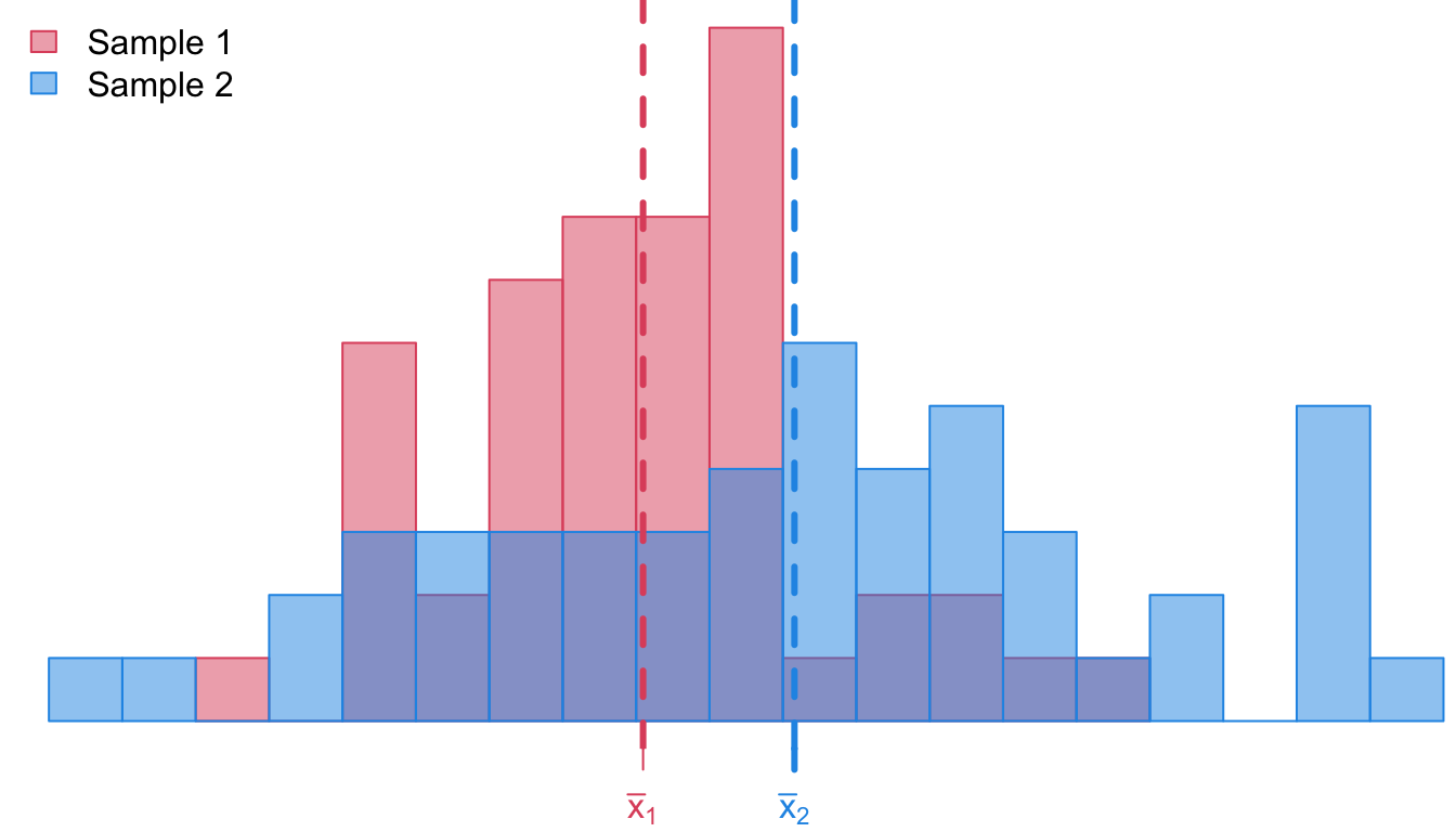
attach(cholesterol)

# Set up the histogram with transparency
hist(before, breaks = 30, col = adjustcolor(2, alpha.f = 0.5), border = 2,
     xlim = range(c(before, after)),
     main = "", xlab = "", ylab = "Frequency")

# Add second histogram
hist(after, breaks = 30, col = adjustcolor(4, alpha.f = 0.5), border = 4, add = TRUE)

# Manually add only the y-axis (removes x-axis numbers)
axis(2)

# Add vertical dashed lines for means
abline(v = mean(before), col = 2, lty = 2, lwd = 2)
abline(v = mean(after), col = 4, lty = 2, lwd = 2)

# Add legend
legend("topright", legend = c("Before", "After"), 
       fill = c(adjustcolor(2, alpha.f = 0.5), adjustcolor(4, alpha.f = 0.5)), 
       border = c(2, 4), bty = "n")

Violin Plot

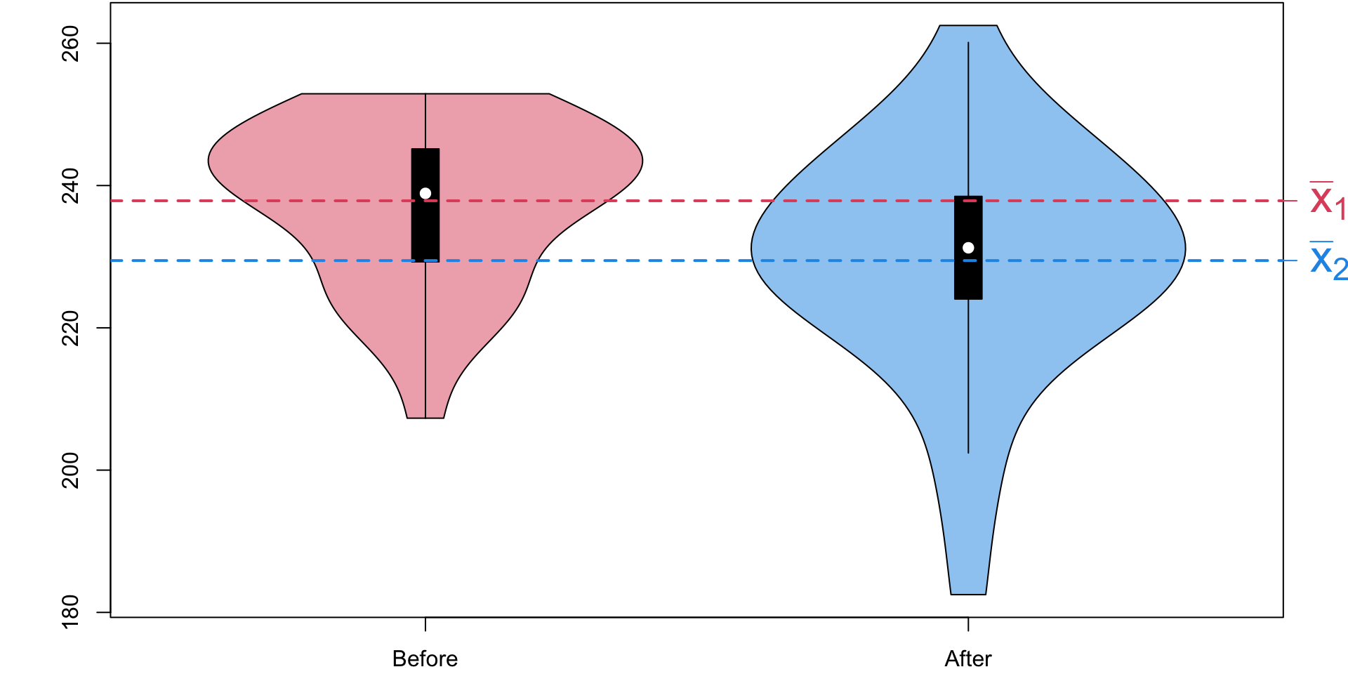
# Load necessary package
library(vioplot)

par(mar=c(2,4,0,2.3)+0.1)
# Create the violin plot
vioplot(before, after, names = c("Before", "After"), 
        col = adjustcolor(c(2, 4), alpha.f = 0.5))


# Add mean points
abline(h=mean(before), col = 2, lwd = 2, lty = 2)  # Mean for "Before"
abline(h=mean(after), col = 4, lwd = 2, lty = 2)   # Mean for "After"

axis(4, at = mean(before), labels = expression(bar(x)[1]), col = 2, col.axis = 2,las = 2, cex.axis  =2)
axis(4, at = mean(after), labels = expression(bar(x)[2]), col = 4, col.axis = 4, las = 2, cex.axis  = 2)

Calculating sample differences

In order to do inference on the paired difference of means,

# Create new column for the differences di
cholesterol$diff =  cholesterol$before - cholesterol$after
head(cholesterol)

Summary statistics

The mean of the differences, \(\bar d\) is:

(dbar = mean(cholesterol$diff))

[1] 8.406667

And the sample standard deviation of the differences is:

(sdd = sd(cholesterol$diff))

[1] 12.46133

The sample size, \(n\), is the number of mathed pairs

(n = nrow(cholesterol))

[1] 30

Normality check

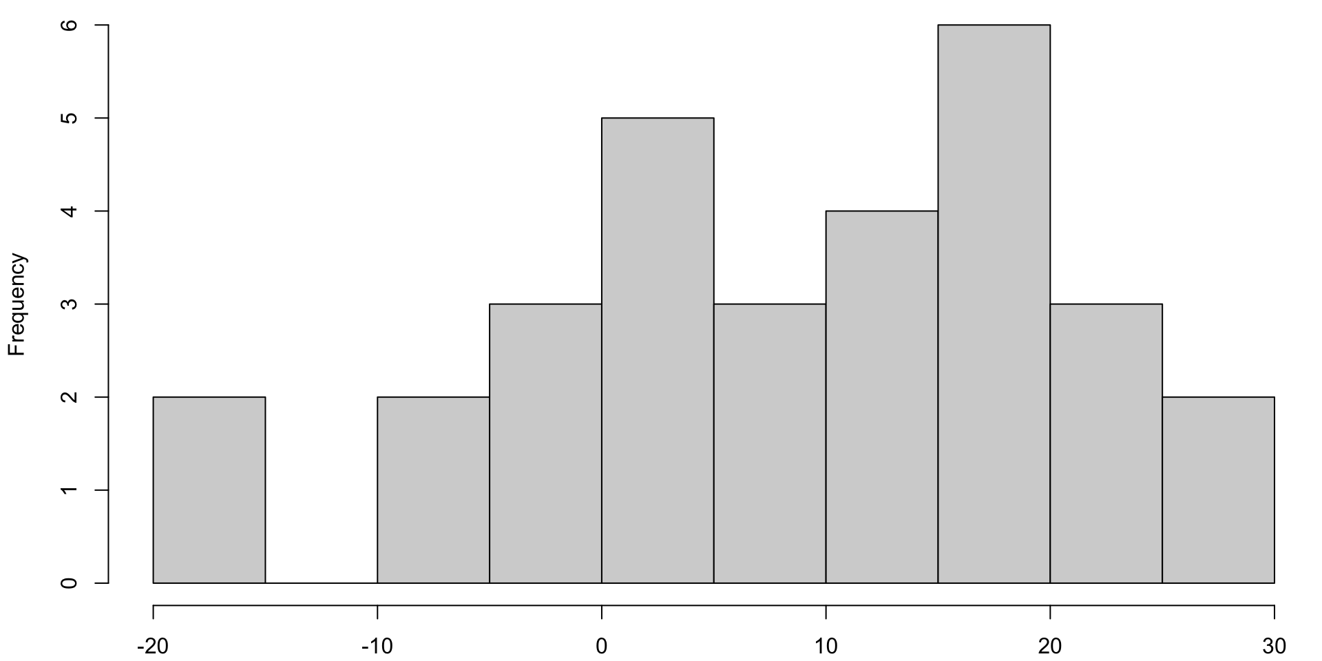
• The test assumes that the differences in cholesterol follow a normal distribution.

• While we have enough data points to rely on the CLT, let’s see how we’d check the normality assumption.

# qq plot
par(mar=c(4,4,4,0)+0.1)
qqnorm(cholesterol$diff)
qqline(cholesterol$diff)

par(mar=c(par.sm))

# histogram of differences
hist(cholesterol$diff, breaks = 10, main = "")

Shapiro-Wilk Test

• Rather than looking at these plots in a subjective way, we could alternative perform a statistical test called the Shapiro-Wilk test for normality.

• The Shapiro-Wilk test is a statistical test used to determine whether a dataset follows a normal distribution.

• It is especially useful for small sample sizes (\(n < 30\)) where visual inspections (e.g., histograms, Q-Q plots) may be less reliable.

Hypotheses for the Shapiro-Wilk Test

• Null Hypothesis (\(H_0\)): The data follow a normal distribution.

• Alternative Hypothesis (\(H_A\)): The data do not follow a normal distribution.

• A low \(p\)-value (< 0.05) suggests that the data significantly deviate from normality.

• A high \(p\)-value (> 0.05) suggests that the data does not significantly deviate from a normal distribution.

We don’t want significance here:

p>0.05 Fail to reject H0: Data are normal (OK for t-test)

p<0.05 Reject H0: Data are not normal (Consider Wilcoxon test)

Shapiro-Wilk Test in R

In R this is conducted using:

shapiro.test(x = cholesterol$diff)

    Shapiro-Wilk normality test

data:  cholesterol$diff
W = 0.9616, p-value = 0.3402

This produces a non-significant \(p\)-value, meaning there is no strong evidence to suggest that the differences in cholesterol deviate from normality.

agian we didn’t really need it since we had a relatively large sample size

iClicker

Hypothesis Test for Cholesterol Reduction

Exercise 2 A nutritionist is investigating whether a new diet reduces cholesterol levels. She measures cholesterol levels before and after the diet for 30 participants.

What are the appropriate null and alternative hypotheses?

1. \(H_0: \mu_d = 0\), \(H_A: \mu_d \neq 0\)
2. \(H_0: \mu_d = 0\), \(H_A: \mu_d > 0\)
3. \(H_0: \mu_d = 0\), \(H_A: \mu_d < 0\)
4. \(H_0: \mu_d \neq 0\), \(H_A: \mu_d = 0\)

Note: we could write \(H_0: \mu_a = \mu_b\) vs. \(H_A: \mu_a < \mu_b\), say, but this is far less common as we typically express our hypothesis as a difference between means.

where \(\mu_b\) and \(\mu_a\) represents that population average cholesterol levels before and after the 8-week diet, respectively.

Test Statistic

\[\begin{align} T &= \dfrac{\bar d - 0}{s_d/\sqrt{n}} \end{align}\] which follows a \(t\)-distribution with \(\nu = n -1 = 29\) d.f. \[\begin{align} t_{obs} &= \dfrac{8.4066667}{12.4613315/\sqrt{30}} = 3.6950473 \end{align}\]

Notice the similarity with the test statistic from one-sample t test: \(\dfrac{\bar x - x_0}{s/\sqrt{n}} \sim t_{\nu = n - 1}\)

iClicker

t-critical

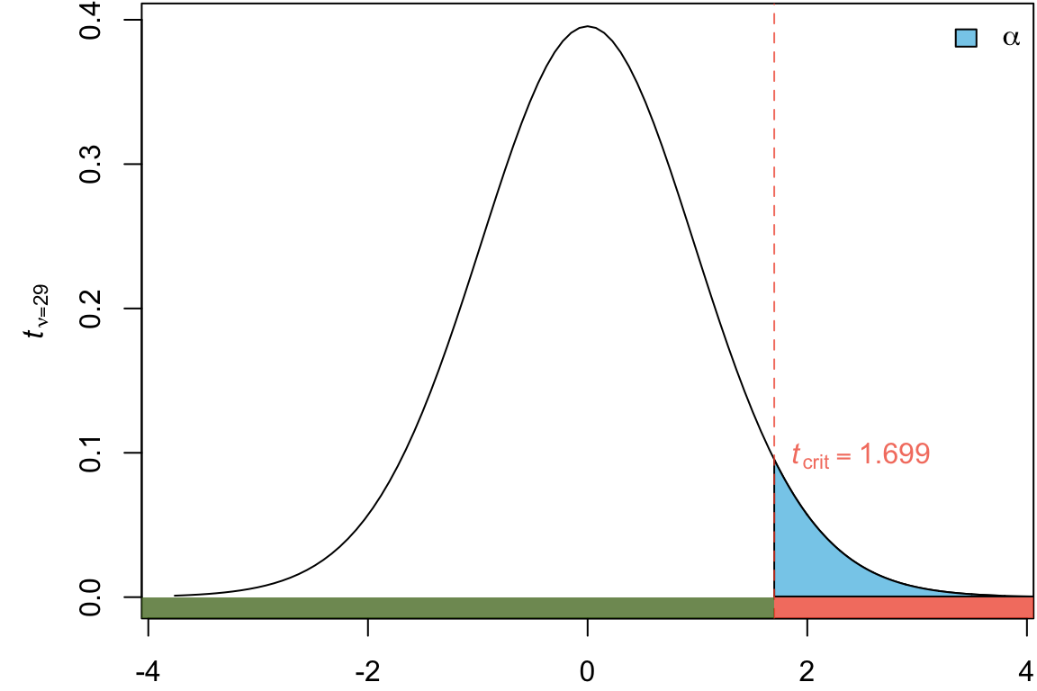
How do we calculate \(t_{crit}\), the critical value for the one-sided test.

qt(0.05, df = n-1, lower.tail = FALSE) 
qt(0.05, df = n-1) 
1 - qt(0.05, df = n-1) 
qt(0.95, df = n-1) 

Critical Value (tables)

The critical value can be found using the table t-table with \(\nu = 29\).

iClicker

Decision based on RR

Does \(t_{obs}\) fall in the rejection region?

1. Yes
2. No

iClicker

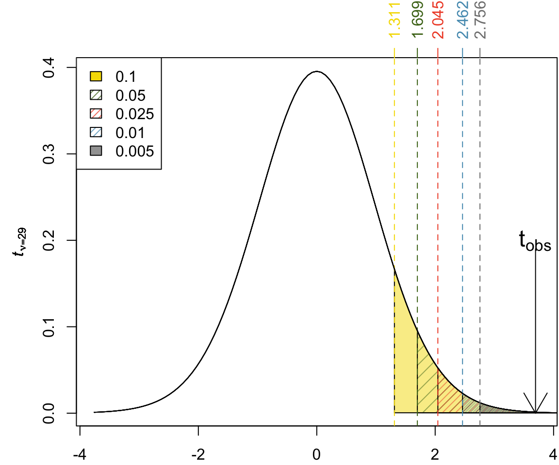
Determining the p-Value from t-Tables

Exercise 3 A paired t-test was conducted to determine whether a new diet reduces cholesterol levels. The test statistic was found to be \(t_{obs} = 3.6950473\) with \(n = 30\) participants. Using a t-table, what is the most accurate way to express the p-value?

1. \(0.01 < p < 0.025\)
2. \(0.025 < p < 0.05\)
3. \(p < 0.01\)
4. \(p > 0.05\)
5. \(p < 0.005\)

p-value

\[\begin{align} &\Pr(t_{29} > t_{obs}) \\ &= \Pr(t_{29} > 3.6950473)\\ &< \Pr(t_{29} > 2.7563859)\\ \implies& p-value < 0.005 \end{align}\]

• Using the t-table for df = 29 (since \(df = n - 1\)), we compare \(|t_{obs}| = 2.45\) to critical values.
  
• From the table:
  • \(t_{0.025, 29} = 2.045\) (p-value 0.05)
  • \(t_{0.01, 29} = 2.462\) (p-value 0.02)
    
• Since \(2.45\) falls between these values, the two-tailed p-value is between 0.02 and 0.05.
• Since this is a one-tailed test (\(H_A: \mu_d < 0\)), we take half of the two-tailed p-value:
  • \(\frac{0.02}{2} = 0.01\), \(\frac{0.05}{2} = 0.025\)
    
  • Thus, \(0.01 < p < 0.025\).
    

p-value

Exact \(p\)-value in R:

pt(3.6950473, df = 29,
          lower.tail = FALSE)

[1] 0.0004547053

Decision

Either can be used to make the decision (should always agree)

1. Based on critical values: Since \(t_{obs} = 3.7 > t_{crit} = 1.7\) (i.e. \(t_{obs}\) falls inside the rejection region), we reject \(H_0\)

2. Based on \(p\)-value: Since \(p\)-value = 4.547^{-4} \(\ll \alpha = 0.05\), we (strongly) reject \(H_0\).

Conclusion: There is strong statistical evidence to suggest that the this 8-week diet plan for lowers cholesterol.

t-test in R

Alternatively, we can conduct this \(t\)-test in R using

t.test(x, y = NULL,
       alternative = c("two.sided", "less", "greater"),
       mu = 0, paired = FALSE, var.equal = FALSE,
       conf.level = 0.95, ...)

alternative = "greater" is the alternative that x has a larger mean than y. For the one-sample case: that the mean is positive.

\(H_0: \mu_x - \mu_y = 0\) vs \(H_0: \mu_x - \mu_y > 0\)

1t.test(x = before,  y = after,
2       alternative = "greater",
3       data = cholesterol,
4       paired = TRUE)

1

\(H_0: \mu_{x} - \mu_{y} = 0\)

2

\(H_A: \mu_{x} - \mu_{y} > 0\)

3

Alternatively we could use x = cholesterol$before, y = cholesterol$after and leave data out.

4

Indicate the data is paired (i.e. matched)¹

where \(\mu_x\) and \(\mu_y\) correspond to the average cholesterol levels before and after the 8-week diet, respectively.

1. Otherwise the wrong test will be performed Welsh test (which assumes independent groups and non-equal variance) is performed

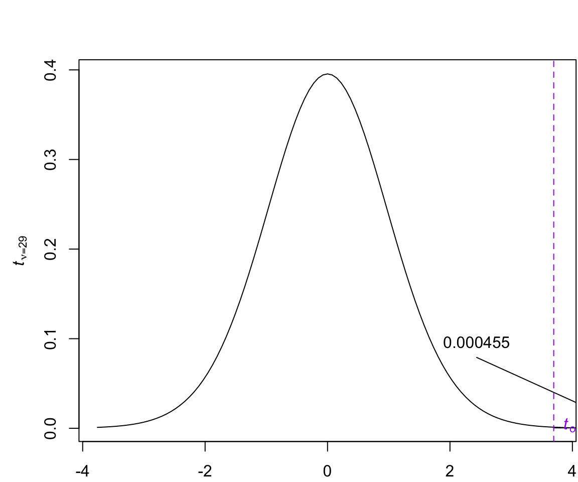
t-table output

t.test(x = cholesterol$before,  y = cholesterol$after,   
       alternative = "greater", paired = TRUE) 

    Paired t-test

data:  cholesterol$before and cholesterol$after
t = 3.695, df = 29, p-value = 0.0004547
alternative hypothesis: true mean difference is greater than 0
95 percent confidence interval:
 4.540953      Inf
sample estimates:
mean difference 
       8.406667 

This output agrees with our \(p\)-value (0.0004547053) and computed observed test statistic (\(t_{obs}=\) 3.6950473)

Comment

• Note for the one-tailed test a one-sided 95% confidence interval¹ is constructed.

• Akin to the relationship between symmetric 95% CI and two-tailed tests, the one-sided confidence interval does provide a decision rule that aligns with the one-tailed test.

  • If the lower bound of the one-sided CI is below \(\mu_0\)​, we fail to reject \(H_0\).

  • If the lower bound is above \(\mu_0\)​, we reject \(H_0\)​.

1. this corresponds to the default conf.level = 0.95

Independent Groups
(equal variance)

Example

Chicken Feed

Exercise 4 An experiment was conducted to measure and compare the effectiveness of various feed supplements on the growth rate of chickens. Newly hatched chicks were randomly allocated into six groups, and each group was given a different feed supplement.

Data

The chickwts is one of the built-in dataset in R.

chickwts # see ?chickwts for more info

Summary Statistics

We will consider a subset of this data set corresponding to the chicks in the soymeal and meatmeal feed supplements.

data <- droplevels(chickwts[chickwts$feed%in%c("soybean", "meatmeal"),])
x1 = soybean = data[data$feed=="soybean",1]
x2 = meatmeal = data[data$feed=="meatmeal",1]
xbar1 = round(mean(x1), 2)
xbar2 = round(mean(x2), 2)
sd1 = round(sd(x1), 2)
sd2 = round(sd(x2), 2)
n1 = length(x1)
n2 = length(x2)

Group	Sample mean	Sample SD	Sample size
soymeal	\(\bar x_1\) = 246.43	\(s_1\) = 54.13	\(n_1 = 14\)
meatmeal	\(\bar x_2\) = 276.91	\(s_2\) = 64.9	\(n_2 = 11\)

[Source] Chicken Weights by Feed Type, (chickwts from the datasets package in R).

Boxplots

par(mar=c(4,5,0,0) + 0.1)
data <- droplevels(chickwts[chickwts$feed%in%c("soybean", "meatmeal"),])
boxplot(weight~feed, data)
# Add jittered points
points(jitter(as.numeric(data$feed)), data$weight, col = "red", pch = 16)

Figure 5: Do these data provide statistically significant evidence that the average weights of chickens that were fed meatmeal and soybean are different?

Violin

# Create violin plot
vioplot(weight ~ feed, data = data, col = "lightblue", 
        main = "Weight by Feed Type", xlab = "Feed Type", ylab = "Weight")

# Add jittered points
points(jitter(as.numeric(data$feed)), data$weight, col = "red", pch = 16)

# Compute and add mean lines
feed_levels <- levels(data$feed)
means <- tapply(data$weight, data$feed, mean)  # Compute means

for (i in 1:length(feed_levels)) {
  lines(c(i - 0.2, i + 0.2), rep(means[i], 2), col = 1, lwd = 2, lty = 2)  # Add mean lines
}

Checking Assumptions

• Independence Within Observations: we a assume that these are a simple random sample of chickens (verified in details; see ?chickwts)

• Independence Between Groups: we assume that the groups of chickens are unpaired.

• Equal Variance Judging by the shapes of the side-by-side boxplot, it appears that the equal variance assumption is reasonable.

Newly hatched chicks were randomly allocated into six groups, and each group was given a different feed supplement. Their weights in grams after six weeks are given along with feed types.

there is no one-to-one match with chicken

Equal variance assumption

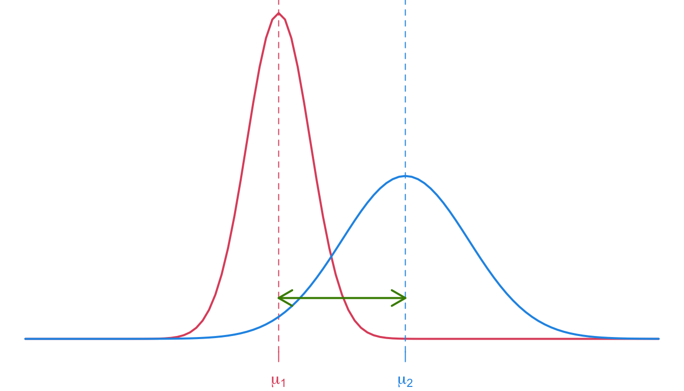
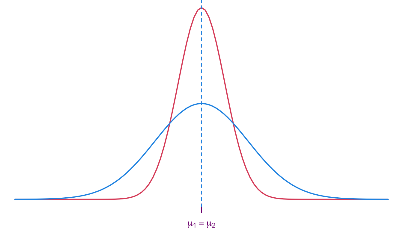
If it is safe to assume \(\sigma^2_1 = \sigma^2_2\), we can carry out the pooled \(t\)-test. We therefore assume Group 1 \(\sim N(\mu_1, \sigma^2)\) and Group 2 \(\sim N(\mu_2, \sigma^2)\).

so rather than distinguishing them, let’s just call it \(\sigma^2\), so that we have

Pooled variance

To estimate this unknown population parameter \(\sigma^2\), we can use a single pooled estimate for this common variance \(\sigma^2\): \[\begin{equation}\label{eq:pooled} s_p^2 = \frac{(n_1 - 1)s_1^2 + (n_2 - 1)s_2^2}{n_1 + n_2 -2} \end{equation}\]

• \(n_i\) is the sample size from Group \(i\) and
• \(s_i\) sample standard deviation from Group \(i\).

Notice how this is simply a weighted average of the two sample variances (weighted by the degrees of freedom). If \(n_1 = n_2\), \(s_p^2\) is simply the average of the two sample variances

Pooled variance

Here’s a function to calculate this in R:

sp <- function(n1, n2, s1, s2, var = FALSE){
    sp2 <- ((n1 - 1)*s1^2 + (n2 - 1)*s2^2)/(n1 + n2 -2)
    if (var){
        return(sp2)
    } else {
        return(sqrt(sp2))
    }
}
pooled_var = sp(n1, n2, sd1, sd2, var = TRUE)
pooled_sd = sqrt(pooled_var)

\[s_p = \sqrt{3487.427813} = 59.0544479\]

see the Summary Statistics slide for calculations of the inputs.

Hypotheses

What is the null and alternative hypothesis?

\[\begin{align} H_0:& \mu_{1} - \mu_{2} = 0 & H_A:& \mu_{1} - \mu_{2} \neq 0 \end{align}\]

Alternative, you may write your hypothesis in words:

• \(H_0\): there is no difference in the long-run average weight of chickens fed with soymeal (\(\mu_1\)) compared to the long-run average weight of chickens fed with meatmeal (\(\mu_2\)).

• \(H_A\): The long-run average weight of chickens fed with soymeal (\(\mu_1\)) is different than the long-run average weight of chickens fed with meatmeal (\(\mu_2\)).

where \(\mu_1\) and \(\mu_2\) represents that long-run average weight of chickens fed soymeal and meatmeal, respectively.

Test stat

\[\begin{equation} \text{Test stat }=\dfrac{\overline{x}_{1} - \overline{x}_{2}}{s_p\sqrt{\frac{1}{n_1} + \frac{1}{n_2}}} \sim t_{n_1 + n_2 -2 = 23} \end{equation}\]

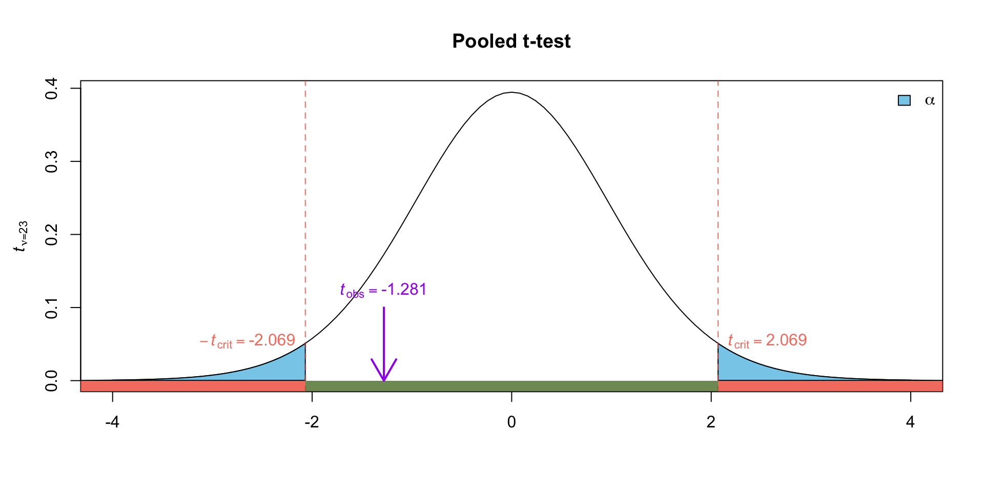
Plugging in our sample statistics and our pooled estimate we get our observed test statistic: \[\begin{equation} t_{obs} =\dfrac{246.43 - 276.91}{59.0544479\sqrt{\frac{1}{14} + \frac{1}{11}}} \approx -1.281 \end{equation}\]

What distribution does the Test stat follow?

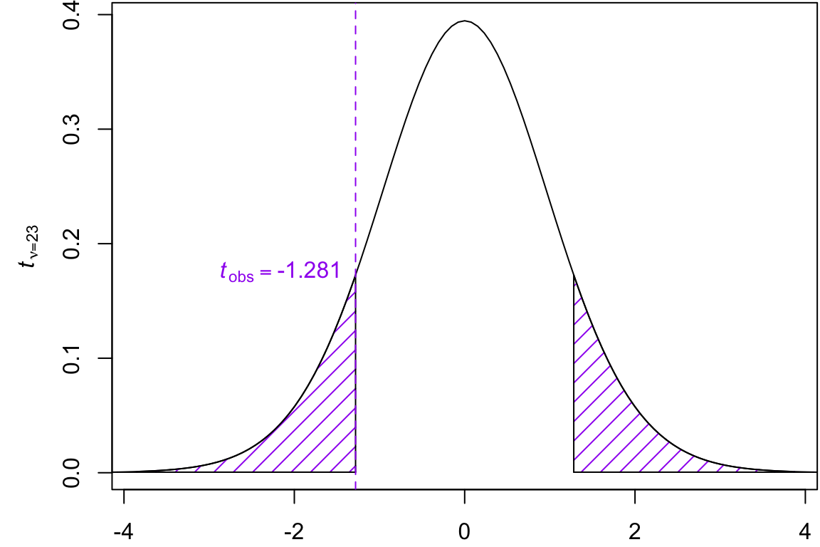
Critical Value

The critical value can be found using the \(t_{\nu = 23}\) distribution.

Find using the table t-table

Critical Value

iClicker

Exercise 5 What is the appropriate code for finding the critical value?

qt(0.025, 23,  lower.tail = FALSE)        #1
qt(0.05, 23,  lower.tail = FALSE)         #2
qt(0.025, 13,  lower.tail = FALSE)      #3
qt(0.025, 24,  lower.tail = FALSE)      #4

p-value

Find the approximate \(p\)-value using the t-table. \(p\)-value = \[\begin{align} &2 \Pr(t_{23} > |t_{obs}|) \\ &2\Pr(t_{23} > 1.281) \end{align}\]

iClicker

Determining the p-Value from t-Tables

The test statistic was found to be \(t_{obs} = -1.2810105\) with \(n = 30\) participants. Using a t-table, what is the most accurate way to express the p-value for the chicken feed example comparing soymeal and meatmeal?

1. \(0.10 < p < 0.25\)
   
2. \(0.25 < p < 0.50\)
   
3. \(p > 0.10\)
   
4. \(p > 0.20\)

p-value

Decision

Since

\[\begin{cases} t_{obs} (=-1.281) \text{ falls outside the rejection region} \\ p\text{-value } (=0.213) > \alpha (=0.05) \end{cases}\]

we fail to reject the null hypothesis, \(H_0\).

Conclusion: there is insufficient evidence to suggest that the long-run average weight of chickens fed with soymeal is different than the long-run average weight of chickens fed with meatmeal.

Since

\[\begin{cases} t_{obs} (=-1.281) \text{ falls inside the rejection region} \\ p\text{-value } (=0.213) < \alpha (=0.05) \end{cases}\]

we reject the null hypothesis in favour of the alternative.

. . .

Conclusion there is sufficient evidence to suggest that the long-run average weight of chickens fed with soymeal is different than the long-run average weight of chickens fed with meatmeal.

pooled t-test in R

t.test(soybean, meatmeal, var.equal = TRUE)

    Two Sample t-test

data:  soybean and meatmeal
t = -1.281, df = 23, p-value = 0.2129
alternative hypothesis: true difference in means is not equal to 0
95 percent confidence interval:
 -79.70142  18.74038
sample estimates:
mean of x mean of y 
 246.4286  276.9091 

which agrees with our previously found \(p\)-value and test statistic.

Verify the CI

Group	Sample mean	Sample SD	Sample size	Pooled
soymeal	\(\bar x_1\) = 246.43	\(s_1\) = 54.13	\(n_1 = 14\)	\(s_p^2 = 59.054^2\)
meatmeal	\(\bar x_2\) = 276.91	\(s_2\) = 64.9	\(n_2 = 11\)

Consulting the summary table, we compute

\[\begin{align} \text{Point estimate } &\pm t_\nu^{\alpha/2} SE\\ \bar x_1 - \bar x_2 &\pm t_{23}^{0.025} \times s_p\sqrt{{1}/{n_1} + {1}/{n_2}}\\ 246.43 - 276.91 &\pm t_{23}^{0.025} \times 23.794\\ -30.48 &\pm 49.221\\ (-79.701 &, 18.741) \end{align}\]

Comment

Note that the slightly different numbers is due to rounding. You can get the exact numbers using the following code:

xbar1 = mean(x1)
xbar2 = mean(x2)
sd1 = sd(x1)
sd2 = sd(x2)

pooled_sd = pooled_var = sp(n1, n2, sd1, sd2)
se = pooled_sd*sqrt(1/n1 + 1/n2)

tcrit = qt(alpha/2, df, lower.tail = FALSE)
ME = tcrit*se
ci = (xbar1 - xbar2)  + c(-1,1)*ME
ci

[1] -79.70142  18.74038

Independent Groups
(unequal variance)

Unequal variance assumption

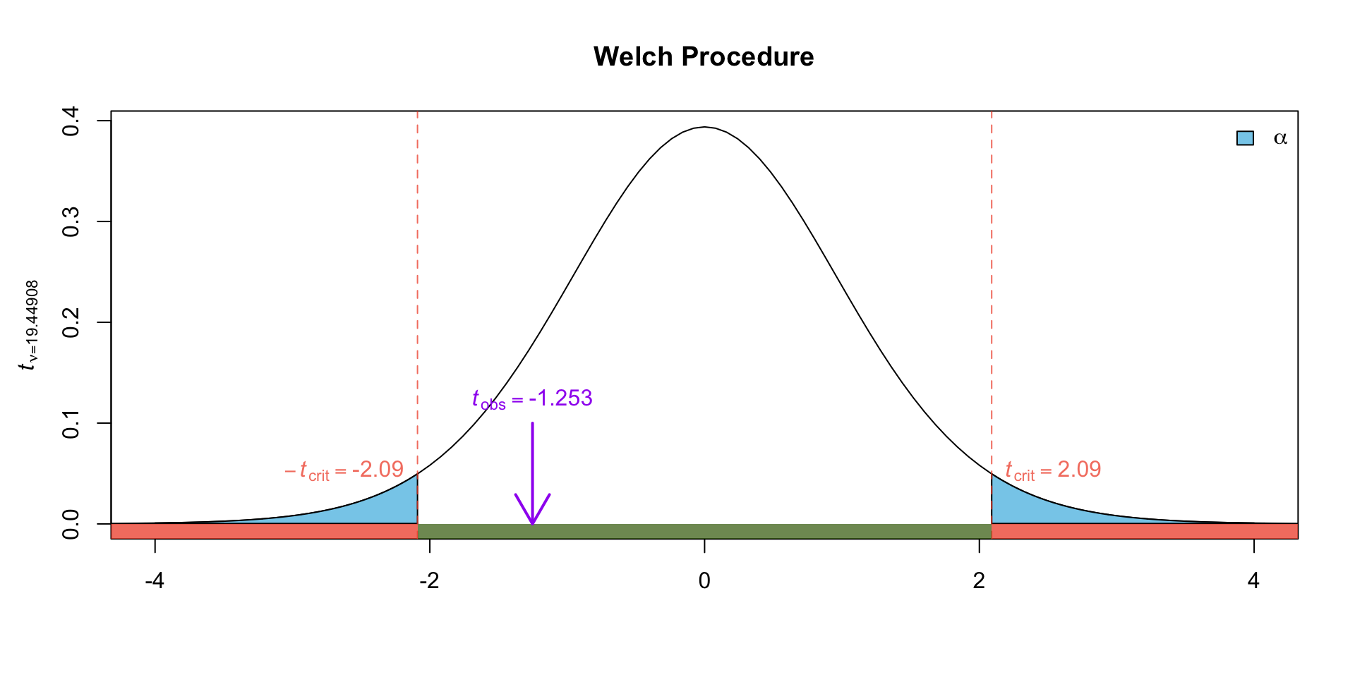
If it is not safe to assume \(\sigma^2_1 = \sigma^2_2\), we can carry out the Welch procedure (approximate \(t\)-test). We therefore assume Group 1 \(\sim N(\mu_1, \sigma_1^2)\) and Group 2 \(\sim N(\mu_2, \sigma_2^2)\).

Welch Procedure

• The Welch procedure is similar to the pooled \(t\)-test, however the test statistic is an approximation even for normal populations (rather than an exact result).

• More importantly, the Welch procedure does not require the assumption of equal population variances.

• While the assumption of equal variance appears reasonable based on the boxplot in Figure 5, let’s carry out the Welch procedure to highlight the difference.

eg. formal F-test for \(H_0: \sigma_1 = \sigma_2\) vs. \(H_A: \sigma_1 \neq \sigma_2\)

Hypotheses and Test statistic

The null and alternative hypothesis will be the same as stated before. The test statistic is now:

\[\begin{equation}\text{Test stat } = \dfrac {\bar{X}_1 - \bar{X}_2 - \delta_0} {\sqrt{ \dfrac{\textcolor{red}{s_1^2}}{n_1} + \dfrac{\textcolor{red}{s_2^2}}{n_2} }} \sim t_{\textcolor{red}{\nu_{w}}} \end{equation}\]

with degrees of freedom found using the formal on the Welch’s degrees of freedom formula (see next slide).

Notice that the SE is different (using the individual sample variance instead of the pooled variance) and the degrees of freedom are different

the pooled estimate won’t be appropriate here anymore since \(\sigma_1\) and \(\sigma_2\) might be very different values so they will be better approximated by their corresponding \(s_1\) and \(s_2\) estimates from the samples

Welch’s degrees of freedom

Group	Sample mean	Sample SD	Sample size
soymeal	\(\bar x_1\) = 246.4285714	\(s_1\) = 54.1290684	\(n_1 = 14\)
meatmeal	\(\bar x_2\) = 276.9090909	\(s_2\) = 64.9006233	\(n_2 = 11\)

The degrees of freedom we use for this test is given by:

\[\begin{align} \nu_w &= \dfrac{\left( \frac{s_1^2}{n_1} + \frac{s_2^2}{n_2} \right)^2}{\frac{1}{n_1 - 1}\left( \frac{s_1^2}{n_1} \right)^2 + \frac{1}{n_2 - 1} \left( \frac{s_2^2}{n_2} \right)^2} = 19.4490812 \end{align}\]

Conservative degrees of freedom

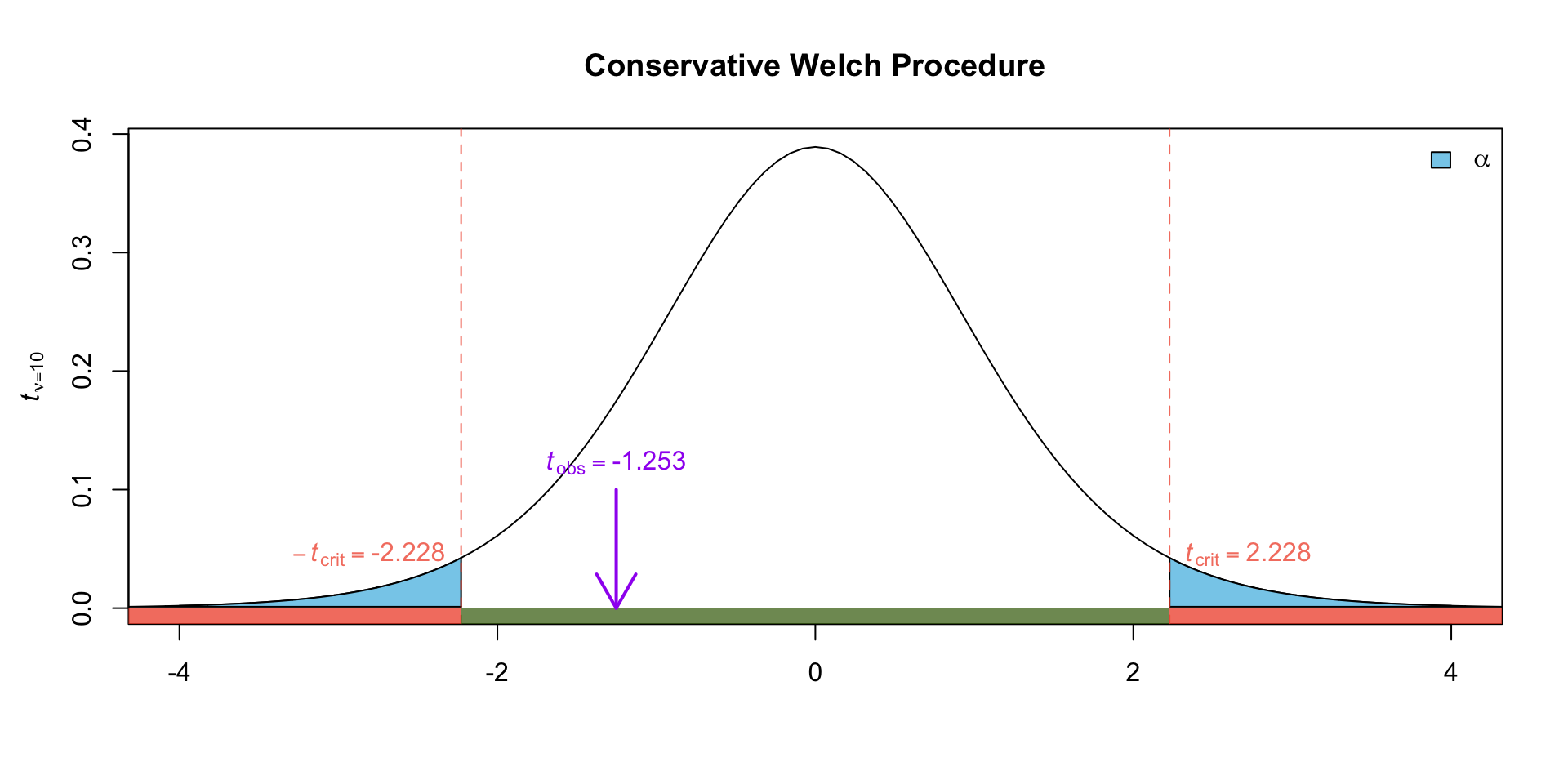
The calculation on the previous page is extremely tedious to do on paper. On a test where you don’t have access to software like R, you may use the following conservative estimate:

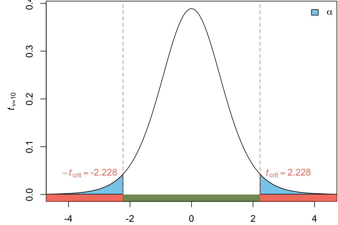
Conservative degrees of freedom for Welch’s Procedure

A conservative estimate for the degrees of freedom for the Welch procedure is

\[ \tilde \nu_w = \min(n_1 -1, n_2-1)\]

Here our \(\tilde \nu_w = \min(14 -1, 11-1) = 10\)

Observed test statistic

Group	Sample mean	Sample SD	Sample size
soymeal	\(\bar x_1\) = 246.4285714	\(s_1\) = 54.1290684	\(n_1 = 14\)
meatmeal	\(\bar x_2\) = 276.9090909	\(s_2\) = 64.9006233	\(n_2 = 11\)

\[\begin{align} t_{obs} &= \dfrac {\bar{x}_1 - \bar{x}_2 - \delta} {\sqrt{\dfrac{s_1^2}{n_1} + \dfrac{s_2^2}{n_2}}}= \dfrac {246.43 - 276.909} {\sqrt{\dfrac{54.13^2}{14} + \dfrac{64.9^2}{11}}} \approx -1.253 \end{align}\]

Be sure to practice obtaining these values on a calculator!

(se_w = sqrt(sd1^2/n1 + sd2^2/n2))
(tobs_w = (xbar1 - xbar2)/se_w)

[1] 24.33516
[1] -1.25253

which is not the same as \(t_{obs} = -1.281\) from the pooled \(t\)-test; see pooled test statistic.

Welch’s Critical value

• Using the Welch’s df, the critical value can be found using the \(t_{\nu_w = 19.4490812}\) distribution.

• Since we will not be using this df on hand-written tests, go ahead and directly calcualte it in R:

var1 = sd1^2; var2 = sd2^2
num_df <- (var1 / n1 + var2 / n2)^2
denom_df <- (var1^2 / (n1^2 * (n1 - 1))) + (var2^2 / (n2^2 * (n2 - 1)))
df_w <- num_df / denom_df
(tcrit_w = qt(alpha/2, df_w, lower.tail = FALSE))

[1] 2.089758

Conservative Critical Value

Using the conservative d.f of 10, the critical value becomes

Find using the table t-table

In R:

df_c = min(c(n1-1,  n2 -1))
(tcrit_c = qt(alpha/2, df_c, 
        lower.tail = FALSE))

[1] 2.228139

Compare the distributions

Compare the distributions

Notice

Compare the distributions

notice for this conservative test (using 10 df instead of 19.4490812) we get a slightly smaller rejection region.

In other word, we’ll need more evidence in order to reject the null hypothesis

p-value

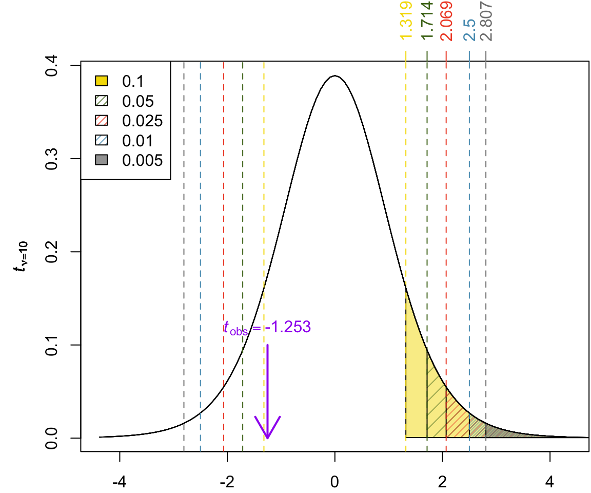
We can find the approximate \(p\)-value using the t-table with the conservative df \(\tilde \nu_w = 10\) \[\begin{align} p\text{-value} = 2\Pr(t_{10} > 1.281)\\ p-value > 0.20 \end{align}\]

The exact \(p\)-value using \(\nu_w =\) 19.449

2*pt(tobs_w, df = df_w) # aka:
2*pt(abs(tobs_w), df=df_w, lower.tail = F)

[1] 0.2252288
[1] 0.2252288

Welch test in R:

t.test(soybean, meatmeal)

    Welch Two Sample t-test

data:  soybean and meatmeal
t = -1.2525, df = 19.449, p-value = 0.2252
alternative hypothesis: true difference in means is not equal to 0
95 percent confidence interval:
 -81.33511  20.37407
sample estimates:
mean of x mean of y 
 246.4286  276.9091 

this agrees with our Welch’s degrees of freedom calculation (\(\nu_w = 19.4490812\)), our Observed test statistic (\(t_{obs} = -1.2525301\))

Comments about Welch

• While the differences were not dramatic in these examples, when the underlining variances \(\sigma_1^2\) and \(\sigma_2^2\) are very different, we begin to see more discrepancy between the solutions.

• The Welch procedure is a more versatile and robust option in many real-world scenarios, since it has one less assumption than the pooled \(t\)-test (which requires \(\sigma_1 = \sigma_2\))

• Recall, however, that the Welch procedure is only an approximate procedure. Hence, you should perform the exact pooled \(t\)-test instead whenever appropriate.

Comments about Pooled

• If in fact \(\sigma_1 = \sigma_2\), pooling the standard deviation in the pooled \(t\)-test allows for a more precise estimation of the standard deviation for each group.

• Another benefit is that the pooled \(t\)-test uses a larger degrees of freedom parameter for the t-distribution (which will lead to narrower CI, and more powerful test)

• Both of these changes may permit a more accurate model of the sampling distribution of \(\bar X_1 - \bar X_2\), if the standard deviations of the two groups are indeed equal.

Guidelines

While formal hypothesis tests for equal variance exist¹, one general rule of thumb² is that if the sample sizes are similar we will require that the variance of one group to be more double the other in order to use the pooled estimate. In other words:

\[ 0.5 < \frac{s_1}{s_2} < 2 \]

1. see the F-test (implemented by var.test() in R).

2. see [Stat 500 Penn State], [BMJ]

Summary

Tests for the difference of population means, i.e. \(H_0: \mu1 - \mu_2 = \delta_0\). All require the normality assumption (which is not very important is the sample sizes are large) and a a simple random sample from the population.

Paired \(t\)-test	Pooled \(t\)-test	Welch
t.test(x,y, paired=T)	t.test(x,y, var.equal = T)	t.test(x,y)
dependent groups	independent groups (\(\sigma_1 = \sigma_2\))	independent groups (\(\sigma_1 \neq \sigma_2\))
\((x_1, y_1), \dots, (x_n, y_n)\) \(d_i = x_i - y_i\)	\((x_1, \dots, x_{n_1})\) , \((y_1, \dots, y_{n_2})\)	\((x_1, \dots, x_{n_1})\) , \((y_1, \dots, y_{n_2})\)
\[\dfrac{\overline{x}_{d} - \delta_0}{\dfrac{s_{d}}{\sqrt{n}}} \sim t_{n-1}\]	\[ \dfrac{\overline{x} - \overline{y} - \delta_0}{\sqrt{\dfrac{s_p^2}{{n_1}}+ \dfrac{s_p^2}{{n_2}}}} \sim t_{n1 + n2 -2} \]	\[ \dfrac{\overline{x} - \overline{y} - \delta_0}{\sqrt{\dfrac{s_1^2}{{n_1}}+ \dfrac{s_2^2}{{n_2}}}} \sim t_{\nu_w} \]

References

“Statistics Online: Courses, Resources, and Materials. (n.d.). Adapted from https://online.stat.psu.edu/stat500/”

Johnson, R. A., I. Miller, and J. E. Freund. 2000. Miller & Freund’s Probability and Statistics for Engineers. Prentice Hall. https://books.google.ca/books?id=yaxQPwAACAAJ.