Lecture 7: Confidence Interval for Variance

STAT 205: Introduction to Mathematical Statistics

Dr. Irene Vrbik

University of British Columbia Okanagan

March 14, 2024

Outline

In this lecture we will be covering

• Chi-squared distribution

• CI for Variance

• Nonparametric Tests: (for median, and sample variance)

Introduction

• Last class we dealt with estimators whos sampling statistics follow a normal distribution (either exactly or approximately thanks to CTL)

• As note previously, many natural phenomena can be modeled adequately by a normal probability distribution.

• In this lecture, we would look into more detail the result of sampling from a normal population when doing inference on the sample population.

Normality is reasonable to assume in many applied problems (when not we’ll deal with other methods for handling that)

Chi-squared

Chi-squared distribution

The PDF of a chi-squared distribution is: \[ f(x; k) = \frac{x^{(k/2) - 1}e^{-x/2}}{2^{k/2}\Gamma(k/2)} \] where \(x >0\), \(\Gamma()\) is the gamma function, and \(k\) is the degrees of freedom.

It is a special case of the gamma distribution. If \(X \sim \chi_{\nu}^2\) and \(c > 0\), then \(cX \sim \Gamma(k = \nu/2, \theta = 2c)\).

The chi-squared distribution often arises in the context of statistics and is used in hypothesis testing and confidence interval construction.

Shape of Chi-squared

Shape:

The chi-squared distribution is positively skewed. The shape of the distribution depends on the degrees of freedom. As k increases, the distribution approaches normality.

Finding probabilities with R

As with the distributions we have seen previously, we could calculate probabilities or quantiles related to the \(\chi^2\) distribution using software like R.

Ex. Find the \(P(\chi^2_{5} < 1.610)\)

pchisq(q=1.610, df = 5) # lower.tail = TRUE (default)

[1] 0.09996259

Ex. Find the \(P(\chi^2_{11} > 18.1)\)

pchisq(q=18.1, df = 11, lower.tail = TRUE) 

[1] 0.9207109

Finding probabilities with tables

Alternatively, you could find probabilities using tables like the one found here.

Ex. Find the \(P(\chi^2_{5} < 1.610)\)

\(1 - P(\chi^2_{5} > 1.610) = 1 - 0.900 = 0.100\)

Ex. Find the \(P(\chi^2_{11} > 18.1)\)

\[ \begin{align} P(\chi^2_{11} > 17.275) > &P(\chi^2_{11} > 18.1) > P(\chi^2_{11} > 19.675)\\ 0.010 > &P(\chi^2_{11} > 18.1) > 0.050 \\ \end{align} \]

Finding quantiles

Find the \(\chi^2_\alpha\) such that \(P(\chi^2_{33} > \chi^2_\alpha) = 0.05\)

In R:

qchisq(p = 0.05, df = 33, lower.tail = FALSE)

[1] 47.39988

From table:

\(P(\chi^2_{40} > 55.758) = 0.05\)

Note on degrees of freedom:

If you don’t see your degrees of freedom on the table, you generally round up to for a more conservative approach.

Rounding up

Lower-tail quantile

Find the \(\chi^2_\alpha\) such that \(P(\chi^2_{12} < \chi^2_\alpha) = 0.05\)

In R:

qchisq(p = 0.05, df=12)

[1] 5.226029

From table: \[ \begin{align} P(\chi^2_{12} < \chi^2_\alpha) = 0.05 \\ = P(\chi^2_{12} > \chi^2_\alpha) = 1 - 0.05\\ \implies \chi^2_\alpha = 5.226 \end{align} \]

Theorem 1

Theorem: Chi-squared

Let \(X_1, X_2, \ldots, X_n\) be be a random sample of size \(n\) from a normal distribution with mean \(\mu\) and variance \(\sigma^2\). Then \(Z_i = \frac{{X_i - \mu}}{{\sigma}}\) are independent, standard normal random variables, \(i = 1, 2, \ldots, n\), and \[ \sum_{i=1}^{n} Z_i^2 = \sum_{i=1}^{n} \left(\frac{{X_i - \mu}}{{\sigma}}\right)^2 \] has a \(\chi^2\) distribution with \(n\) degrees of freedom.

Wackerly - 356 Chapter 7

Proof: Because \(X_1, X_2, \ldots, X_n\) is a random sample from a normal distribution with mean \(\mu\) and variance \(\sigma^2\), Example 6.10 (\(Z = \frac{X-\mu}{\sigma} \sim N(0,1)\) implies that \(Z_i = \frac{{X_i - \mu}}{{\sigma}}\) has a standard normal distribution for \(i = 1, 2, \ldots, n\).

Further, the random variables \(Z_i\) are independent because the random variables \(X_i\)’s are independent, \(i = 1, 2, \ldots, n\). The fact that \(\sum_{i=1}^{n} Z_i^2\) has a \(\chi^2\) distribution with \(n\) df follows directly from Theorem 6.4.

Proof Theorem 6.4: Because \(X_i\) is normally distributed with mean \(\mu_i\) and variance \(\sigma_i^2\), the result of Example 6.10 implies that \(Z_i\) is normally distributed with mean \(0\) and variance \(1\). From Example 6.11, we then have that \(Z_i^2\) is a \(\chi^2\)-distributed random variable with \(1\) degree of freedom. Thus, \[ mZ_i^2(t) = (1 - 2t)^{-1/2}, \] and from Theorem 6.2, with \(V = \sum_{i=1}^{n} Z_i^2\), \[ mV(t) = mZ_1^2(t) \times mZ_2^2(t) \times \ldots \times mZ_n^2(t) = (1 - 2t)^{-1/2} \times (1 - 2t)^{-1/2} \times \ldots \times (1 - 2t)^{-1/2} = (1 - 2t)^{-n/2}. \] Because moment-generating functions are unique, \(V\) has a \(\chi^2\) distribution with \(n\) degrees of freedom.

Theorem 2

Pivot for Sample variance

Let \(X_1, X_2, \ldots, X_n\) be a random sample from a normal distribution with mean \(\mu\) and variance \(\sigma^2\). Then \[ \frac{{(n - 1)S^2}}{{\sigma^2}} = \frac{1}{{\sigma^2}} \sum_{i=1}^{n} (X_i - \bar{X})^2 \] has a \(\chi^2\) distribution with \((n - 1)\) degrees of freedom. Also, \(\bar{X}\) and \(S^2\) are independent random variables.

proof is quite involved - a simpler proof can be seen on page 358 or wackerly

A pivotal quantity or pivot is a function of observations and unobservable parameters such that the function’s probability distribution does not depend on the unknown parameters

CI

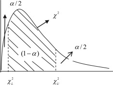
Find two numbers, \(\chi_L^2\) and \(\chi_U^2\), such that: The foregoing inequality can be rewritten as: \[ P\left(\chi_L^2 \leq \frac{(n-1)S^2}{\sigma^2} \leq \chi_U^2\right) = 1 - \alpha. \] The foregoing inequality can be rewritten as: \[ P\left(\frac{(n-1)S^2}{\chi_U^2} \leq \sigma^2 \leq \frac{(n-1)S^2}{\chi_L^2}\right) = 1 - \alpha. \] Hence, a \((1 - \alpha) \times 100\%\) confidence interval for \(\sigma^2\) is given by \[ \left( \frac{(n-1)S^2}{\chi_U^2}, \frac{(n-1)S^2}{\chi_L^2} \right) \] For convenience, we take the areas to the right of \(\chi_U^2\) and to the left of \(\chi_L^2\) to be both equal to \(\alpha/2\).

CI cont’d

CI for Variance

If \(\bar{X}\) and \(S\) are the mean and standard deviation of a random sample of size \(n\) from a normal population, then: \[ P\left(\frac{(n - 1)S^2}{\chi_{\frac{\alpha}{2}}^2} \leq \sigma^2 \leq \frac{(n - 1)S^2}{\chi_{1 - \frac{\alpha}{2}}^2}\right) = 1 - \alpha, \] where the \(\chi^2\) distribution has \((n - 1)\) degrees of freedom.

That is, we are \((1 - \alpha) \times 100\%\) confident that the population variance \(\sigma^2\) falls in the interval \[ \left(\frac{(n - 1)S^2}{\chi_{\frac{\alpha}{2}}^2}, \frac{(n - 1)S^2}{\chi_{1 - \frac{\alpha}{2}}^2}\right), \]

Example

Example: sample variance 90% CI

A random sample of size 21 from a normal population gave a standard deviation of 9. Determine a 90% CI for \(\sigma^2\).

Here \(n = 21\) and \(s^2 = 81\). From the \(\chi^2\) table with 20 degrees of freedom,
\[ \begin{align} \chi_L^2 &= \chi^2_{\frac{\alpha}{2}} = \chi^2_{0.10/2} = \chi^2_{0.05}\\ \chi_U^2 &= \chi^2_{1 - \frac{\alpha}{2}} = \chi^2_{1 - 0.10/2} = \chi^2_{0.95} \end{align} \]

Therefore, a 90% confidence interval for \(\sigma^2\) is obtained from:

\[ \left(\frac{(n - 1)S^2}{\chi_{\frac{\alpha}{2}}^2}, \frac{(n - 1)S^2}{\chi_{1 - \frac{\alpha}{2}}^2}\right). \] Thus we have: \[ \frac{(20)(81)}{31.4104} < \sigma^2 < \frac{(20)(81)}{10.8508}, \] or we are 90% confident that \(51.575 < \sigma^2 < 149.298\).

Procedure

Chapter 5 of (Ramachandran and Tsokos 2020)

Example: Cholesterol

Cholesterol Example

The following data represent cholesterol levels (in mg/dL) of 10 randomly selected patients from a large hospital on a particular day:

data = c(360,352,294,160,146,142,318,200,142,116)

Determine a 95% CI for \(\sigma^2\).

Checking Normality

boxplot(data)

library(car)
qqnorm(data);qqline(data)

Even though the scattergram does not appear to follow a straight line, the data are still within the band, so we can assume approximate normality for the data. (In situations like this, it is more appropriate to use nonparametric tests explained in Chapter 12.) A box plot of the data shows that there are no outliers.

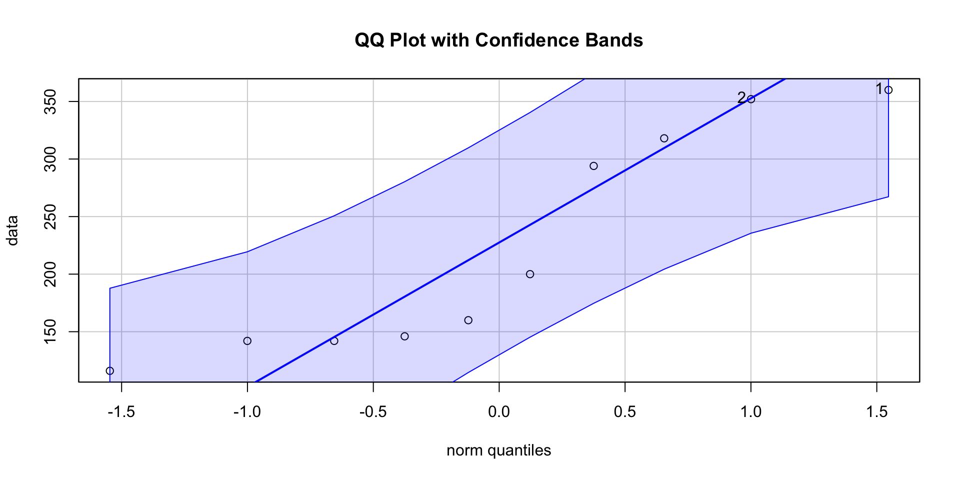
QQ plot with bands

library(car)
# Create QQ plot with 95% confidence bands
qqPlot(data, main = "QQ Plot with Confidence Bands", envelope = 0.95)

[1] 1 2

https://online.stat.psu.edu/stat500/lesson/5/5.4/5.4.4

Since the points all fall within the confidence limits, it is reasonable to suggest that the data come from a normal distribution.

Comment

• In this situation it might be better to do a nonparametric confidence interval as the normality checks are suspect.

• For now since the data are still within the band, so we can assume approximate normality for the data.

Solution assuming normality

From the \(\chi^2\) table, \(\chi^2_{\text{L}}\) and \(\chi^2_{\text{U}}\) are found. Therefore, a 90% confidence interval for \(\sigma^2\) is obtained from: \[ \left( \frac{{(n - 1)S^2}}{{\chi^2_{\alpha/2, n-1}}}, \frac{{(n - 1)S^2}}{{\chi^2_{1-\alpha/2, n-1}}} \right) \] Thus we get: \[ \left( \frac{{(9)(96.9^2)}}{{\chi^2_{9, 19.023}}}, \frac{{(9)(96.9^2)}}{{\chi^2_{9, 2.70}}} \right) \] or we are 95% confident that \(4442.3 < \sigma^2 < 31,299\).

Note that the numbers look very large, but it is the value of variance. By taking the square root of the numbers on the both sides, we can also get a CI for the standard deviation σ.

Comment

• These numbers look very large; these are variance value (the average of the squared differences from the mean).

• By taking the square root of the numbers on the both sides, we can also get a CI for the standard deviation \(\sigma\).

• The CI for the standard deviation is given by:

\[ \begin{align} \sqrt{4442.3} < \sigma < \sqrt{31,299}\\ 66.6505814 < \sigma < 176.9152339 \end{align} \]

Parametric Tests:

• The CI for sample variance are based on the assumption that the sample(s) come from a normal population

• In general, parameter test assume that the sample comes from a population having some specified population probability distribution(s) with free parameters.

• These are generally more powerful when underlying assumptions are met.

• However, assumptions are hard to verify, especially for small sample sizes or ordinal scale data.

Why not use nonparametric methods all the time? The answer lies in the fact that when the assumptions of the parametric tests can be verified as true, parametric tests are generally more powerful than nonparametric tests.

Nonparametric Tests:

• Tests that do not make distributional assumptions

• These are ideal when a distributional model for data is unavailable or when dealing with non-normal data.

Why not use nonparametric methods all the time?

• When the assumptions of the parametric tests can be verified, parametric tests are generally more powerful.

• Because only ranks are used in nonparametric methods, information is lost; hence the loss of power

no assumptions like the usual assumption of normality.

loss of info because ranks (instead of actual values) are used

nonparametric procedures cannot be as powerful as their parametric counterparts when parametric tests can be used.

Distribution-Free Tests:

• Distribution-free tests are a subset of non-parametric tests

• Include tests that do not involve population parameters, such as testing whether the population is normal.

• Generally make weak assumptions like equality of population variances and/or the distribution.

• Most of the nonparametric procedures involve ranking data values and developing testing methods based on the ranks.

Use of median

• In a nonparametric setting, we need procedures where the sample statistics used have distributions that do not depend on the population distribution.

• The median is commonly used as a parameter in nonparametric settings.

• We assume that the population distribution is continuous.

Theoretical developments can be found in many specialized books on the subject.

For brevity and clarity, this chapter is presented without much theoretical explanation to focus on the methods

Nonparameter CI (setup)

Let \(M\) denote the median of a distribution and \(X\) (assumed continuous) be any observation from that distribution. Then,

\[P(X \leq M) = P(X \geq M) = \frac{1}{2}\]

This implies that, for a given random sample \(X_1, \ldots, X_n\) from a population with median \(M\), the distribution of the number of observations falling below \(M\) will follow a binomial distribution with parameters \(n\) and \(\frac{1}{2}\), irrespective of the population distribution.

Binomial distribution

• Let \(N^-\) be the number of observations less than \(M\).

• Then the distribution of \(N^-\) is binomial with parameters \(n\) and \(\frac{1}{2}\) for a sample of size \(n\).

• Hence, we can construct a confidence interval for the median using the binomial distribution.

For a given probability \(\alpha\), we can determine \(a\) and \(b\) such that \[\begin{align*} P(N^- \leq a) &= \sum_{i=0}^{a} \binom{n}{i} \left(\frac{1}{2}\right)^i \left(\frac{1}{2}\right)^{n-i} \\ &= \sum_{i=0}^{a} \binom{n}{i} \left(\frac{1}{2}\right)^n = \frac{\alpha}{2}\\ P(N^- \geq b) &= \sum_{i=b}^{n} \binom{n}{i} \left(\frac{1}{2}\right)^i \left(\frac{1}{2}\right)^{n-i} \\ &= \sum_{i=b}^{n} \binom{n}{i} \left(\frac{1}{2}\right)^n = \frac{\alpha}{2}. \end{align*}\]

Comment

• If exact probabilities cannot be achieved, choose \(a\) and \(b\) such that the probabilities are as close as possible to the value of \(\alpha/2\).
• Furthermore, let \(X(1), X(2),\dots, X(a)\),\(\dots\), \(X(b), \dots, X(n)\) be the order statistics of \(X_1,\dots, X_n\) as depicted below

Figure 12.2 from (Ramachandran and Tsokos 2020)

Interval

• Then the population median will be above the order statistic, \(X_{(b)}, \left(\frac{\alpha}{2}\right)_{100\%}\) of the time and below the order statistic, \(X_{(a)}, \left(\frac{\alpha}{2}\right)_{100\%}\) of the time.

• Hence, \((1-\alpha)100%\) confidence interval for the median of a population distribution will be \[ X_{(a)} < M < X_{(b)}. \]

• Which we can write as \(P\left(X_{(a)} < M < X_{(b)}\right) \geq 1 - \alpha.\)

• By dividing the upper and lower tail probabilities equally, we find that \(b = n + 1 - \alpha\).

• Therefore, the confidence interval becomes

\[ X_{(a)} < M < X_{(n + 1 - a)}. \]

• In practice, \(a\) will be chosen so as to come as close to attaining \(\frac{\alpha}{2}\) as possible.

Procedure

From Section 12.2 of (Ramachandran and Tsokos 2020)

Example

Example: car

In a large company, the following data represent a random sample of the ages of 20 employees.

data = c(24,31,28,43,28,56,48,39,52,32,38,49,51,49,62,33,41,58,63,56)

Construct a 95% confidence interval for the population median M of the ages of the employees of this company.

Let’s first store the order data in:

(sdat <- sort(data))

 [1] 24 28 28 31 32 33 38 39 41 43 48 49 49 51 52 56 56 58 62 63

Step 2

Instead of using binomial tables (eg here) we’ll find these in R

n <- 20; alpha <- 0.05  
# Calculate cumulative probabilities for successes 1 to 6
cumulative_probabilities <- pbinom(1:6, n, prob = 0.5, lower.tail = TRUE)

knitr::kable(rbind(x = 1:6, px= format(round(cumulative_probabilities,4))))

x	1	2	3	4	5	6
px	0.0000	0.0002	0.0013	0.0059	0.0207	0.0577

For \(X\sim Bin(20, 0.5)\) we see \(P(X \leq 5) = 0.0207\). Hence, \(a = 5\) comes closest to achieving \(\alpha/2 = 0.025\).

This will find the value of \(a\) that obtains at least \(\alpha/2\) prob

qbinom(alpha/2, n, prob = 0.5, lower.tail = TRUE) # 6

Step 3

Hence, in the ordered data, we should use the fifth observation,

sdat[5]

[1] 32

for the lower confidence limit and the 16th observation (\(n + 1–a = 21–5 = 16\)),

sdat[16]

[1] 56

for the upper confidence limit.

Step 4

Therefore, an approximate 95% confidence interval for \(M\) is \[ 32 < M < 56 \]

Thus, we are at least 95% certain that the true median of the employee ages of this company will be greater than 32 and less than 56, that is, \[ P\left(32 < M < 56\right) \geq 0.95. \]

Non-parmetric CI for sample variance

• A non-parametric confidence interval for the sample variance typically involves using resampling methods, such as bootstrapping.

• The bootstrap method is a non-parametric statistical technique that involves repeatedly resampling with replacement from the observed data to estimate the sampling distribution of a statistic.

Procedure

1. Collect the Data: Obtain your sample data, denoted as \(X_1, X_2, \dots, X_n\)

2. Bootstrap Resampling:

   • Randomly sample with replacement from the observed data to create a resampled dataset.

   • Calculate the sample variance for each resampled dataset.

3. Repeat the Resampling: Repeat the resampling process \(B\) times, where \(B\) is a large number (e.g., 1000 or more).

4. Calculate Confidence Interval: From the distribution of the resampled sample variances, calculate the desired percentile-based confidence interval. For example, you might use the 2.5th percentile to the 97.5th percentile for a 95% confidence interval.

5. Result: The resulting interval is the non-parametric confidence interval for the sample variance.

Here’s a general outline of how you might construct a non-parametric confidence interval for the sample variance using bootstrapping:

Cholestoral Ex Returned

Returning to Example: Cholesterol, we can find the corresponding CI for the sample variance using the non-parameter bootstrap technique.

data = c(360,352,294,160,146,142,318,200,142,116)

Set a see for reproducibility, and create a function for calculating sample variance

# Assuming your sample data is stored in 'data'
set.seed(123)  # for reproducibility
B <- 1000  # number of bootstrap samples


# Function to calculate sample variance
calculate_sample_variance <- function(x) {
  return(var(x)) # using n-1 in denominator
}

we don’t need to make a function but i’m trying to keep it generic

Use replicate() to take

# Bootstrap resampling
bootstrap_variances <- replicate(B, calculate_sample_variance(sample(data, replace = TRUE)))

# Calculate confidence interval
confidence_interval <- quantile(bootstrap_variances, c(0.025, 0.975))

# Print the result
cat("Non-parametric 95% Confidence Interval for Sample Variance:", confidence_interval, "\n")

Non-parametric 95% Confidence Interval for Sample Variance: 4157.674 12116.45 

Compared with the earlier result of:

\[4442.3 < \sigma^2 < 31,299\]

1. sample(data, replace = TRUE): This part randomly samples from the data vector with replacement. The replace = TRUE argument indicates that each element is drawn independently with replacement, meaning that the same element can be sampled more than once.

2. calculate_sample_variance(...): This part calculates the sample variance for the resampled data. The calculate_sample_variance function is assumed to be a custom function that takes a vector of data as input and returns its sample variance.

3. replicate(B, ...): This part replicates the entire process B times. It repeatedly performs the resampling and variance calculation, creating a vector of sample variances.

And for sd…

Similarly we could do this for standard deviation.

calculate_sample_sd <- function(x) {return(sqrt(var(x)))}
bootstrap_variances <- replicate(B, calculate_sample_sd(sample(data, replace = TRUE)))
confidence_interval <- quantile(bootstrap_variances, c(0.025, 0.975))

# Print the result
cat("Non-parametric 95% Confidence Interval for Sample Standard deviation:", confidence_interval, "\n")

Non-parametric 95% Confidence Interval for Sample Standard deviation: 60.83901 110.3372 

Compare with the earlier CI for standard deviation is given by:

\[ \begin{align} 66.651 < \sigma < 176.915 \end{align} \]

References

Ramachandran, K. M., and C. P. Tsokos. 2020. Mathematical Statistics with Applications in r. Elsevier Science. https://books.google.ca/books?id=t3bLDwAAQBAJ.