Lecture 6: Confidence Intervals for Means and Proportions

STAT 205: Introduction to Mathematical Statistics

Dr. Irene Vrbik

University of British Columbia Okanagan

Introduction

• Last lecture used the MM and MLE to derive point estimates (e.g. \(\bar x\), \(s^2\), \(\hat \beta\)) for population parameters (e.g. \(\mu\), \(\sigma^2\), \(\beta\)) .

• A single estimate does not provide information about the reliability or uncertainty associated with the estimator.

• Since the sampling distribution tells us how much the sample statistic (e.g., \(\bar{X}\)) varies from sample to sample, we can use it to construct an interval that likely contains the true population parameter.

MM = method of moments, MLE = maximum likelihood estimation

Outline

Using our knowledge of sampling distributions we derive:

• Confidence intervals for \(\mu\)

• Confidence intervals for \(p\)

• Confidence intervals for \(\sigma^2\)

In this lecture we will be covering interval estimators (i.e. confidence intervals), a powerful tool that not only provides point estimates but also offers insights into the range of likely values.

Confidence Interval

A confidence interval (CI) is an interval estimate of a population parameter based on a sample statistic and its sampling distribution.

• A confidence interval (CI) provides an interval or range of plausible values for the population parameter.

• It is constructed using a sample statistic and its sampling distribution.

• CI provides some prescribed degree of confidence (C) of securing the true parameter (typically 90%, 95%¹, or 99%)

• A higher confidence level results in a wider interval.

1. in this course, unless otherwise specified you should assume 95%

Comments

\(L\) and \(U\) will be used to denote¹ the lower and upper confidence limits, respectively.

For this interval \((L, U)\) to be useful,

1. the true population parameter \(\theta\) should have a high probability of falling between \(L\) and \(U\)
2. the length of the interval should be relatively narrow

1. this notation is not standard across textbooks

Garfield Comic Strip

Normal Distribution

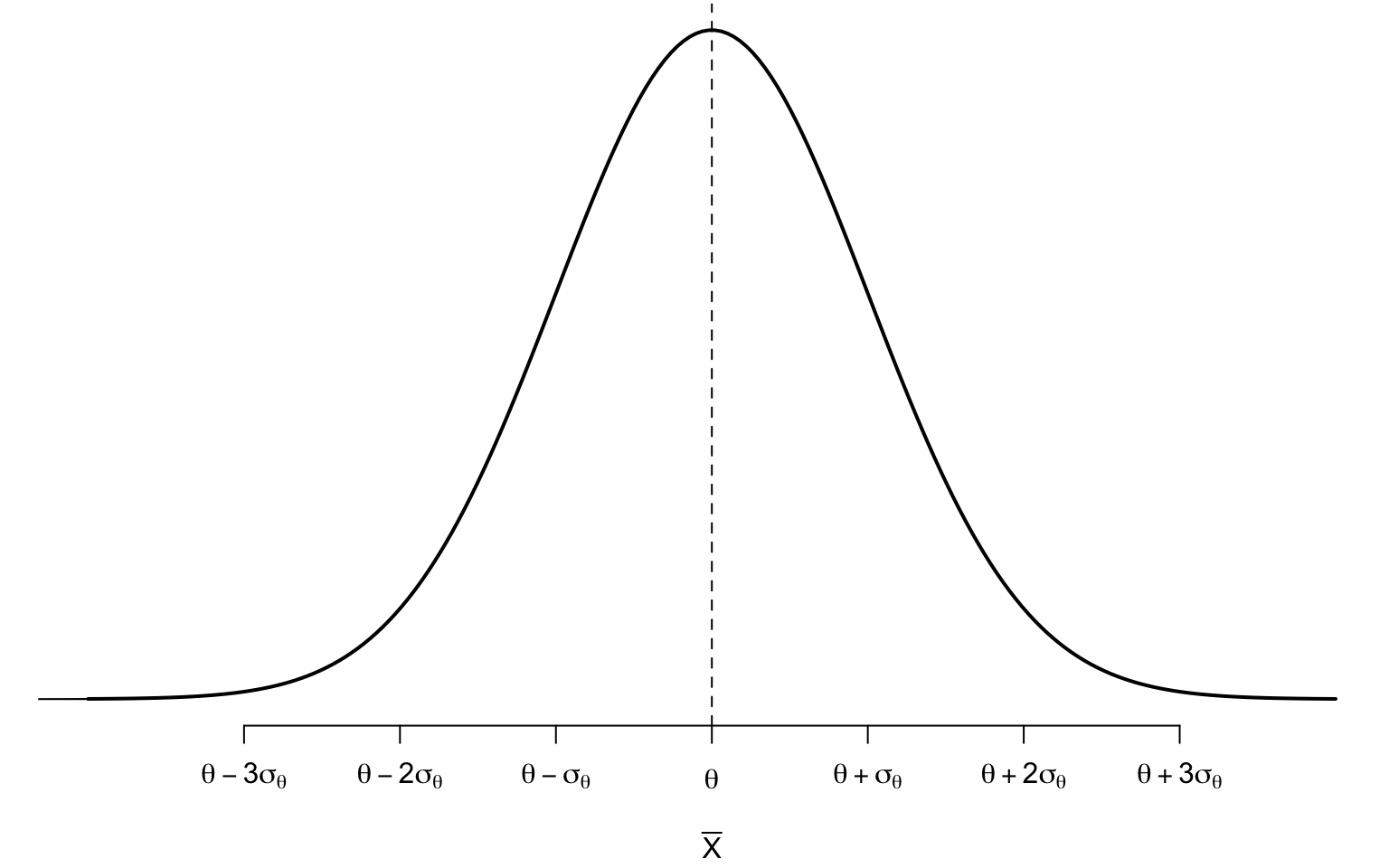
For the normal distribution, 95% of observations are within 1.96 standard deivations of the distribution’s center.

a large number of values (68%)from this distribution will be included withone one sd of the mean

Constructing confidence intervals

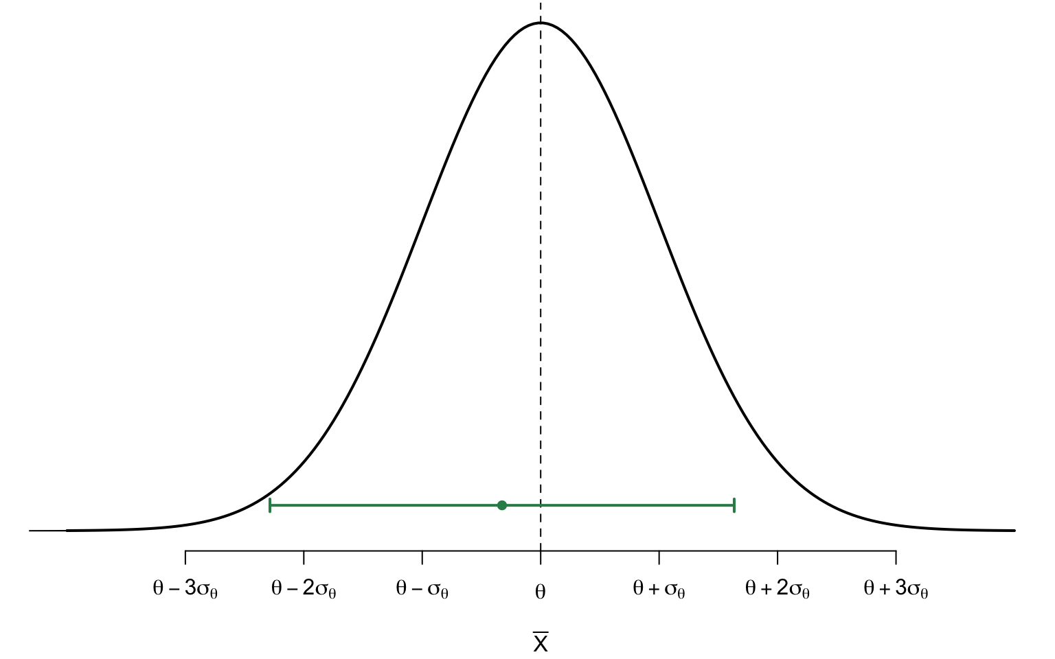
Using this principle, if a point estimator can be modeled using a normal distribution, we can construct a plausible range of values for a parameter by looking with 1.96 standard errors¹ of the point estimate.

\[ \text{point estimate} \pm 1.96 \times SE \]

where SE stands for the standard error of the point estimate.

1. recall that standard error (SE) is the standard deviation of a sample statistic.

Constructing confidence intervals

\[ \text{point estimate} \pm \textcolor{red}{\boxed{1.96 \times SE}} \phantom{asdflj} \]

\[ \phantom{\text{point estimate} \pm } \textcolor{red}{\boxed{\text{Margin of Error}}} \]

The so-called margin of error is a measure of the precision or uncertainty associated with the estimate derived from a sample.

Therefore, the smaller we can get this number, the better!

While decreasing the value of z∗ will also achieve a decrease in m, doing so will decrease our confidence level.

Deriving a CI

Consider the sample mean \(\overline{X} \sim N(\mu, SE_{\overline{X}} = \sigma/\sqrt{n})\). It follows:

\[ \begin{align} \frac{\overline{X} - \mu}{\sigma/\sqrt{n}} \sim N(0,1) \end{align} \]

\[ \begin{align*} P \left( -1.96 < \frac{(\overline{X} - \mu)}{\sigma/\sqrt{n}} < 1.96 \right) = 0.95\\ P \left( -1.96\frac{\sigma}{\sqrt{n}} < \overline{X} -\mu < 1.96 \frac{\sigma}{\sqrt{n}}\right) = 0.95\\ P \left( 1.96 \frac{\sigma}{\sqrt{n}} > \mu - \overline{X} > - \frac{\sigma}{\sqrt{n}} 1.96 \right) = 0.95\\ P \left(\overline{X} -1.96\frac{\sigma}{\sqrt{n}} < \mu < \overline{X} + 1.96 \frac{\sigma}{\sqrt{n}}\right) = 0.95\\ \end{align*} \]

CI Definition

100(C) Confidence Interval

A \(100(C)\)% confidence interval for \(\mu\) is given in the form

\[ \begin{align} \bar{x} \ &\pm m & \text{ or} \\ (\bar{x} - m &, \bar{x} + m) \end{align} \]

• where \(m\) is called the margin of error given by \(z^* \sigma/\sqrt{n}\)

• \(z^*\) is the value such that \(P(-z^* < Z < z^*) = C\)

Finding z*

To find the \(z^*\) in R, you can use the qnorm() function

alpha = 0.05
qnorm(1-alpha/2)

[1] 1.959964

While the lower z-critical score is just the negative version of the number calculated above, for demonstration purposes lets also compute it in R:

qnorm(alpha/2)

[1] -1.959964

From a table ..

iClicker: finding \(z^*\)

What is the \(z^*\) for a 98% confidence interval?

1. 2.33

2. 2.05

3. 2.58

4. None of the above

Note

The sign of the \(z^*\) doesn’t matter since the standard normal is a symmetric distribution about 0

Warning

Warning

For this CI to be exact, we must have the following:

1. The sample data must be a simple random sample from the population of interest
2. The population must be normally distributed

When it is not guaranteed that our population is normal, this interval is approximate for large \(n\) (thanks to the CLT)

Why “confidence”

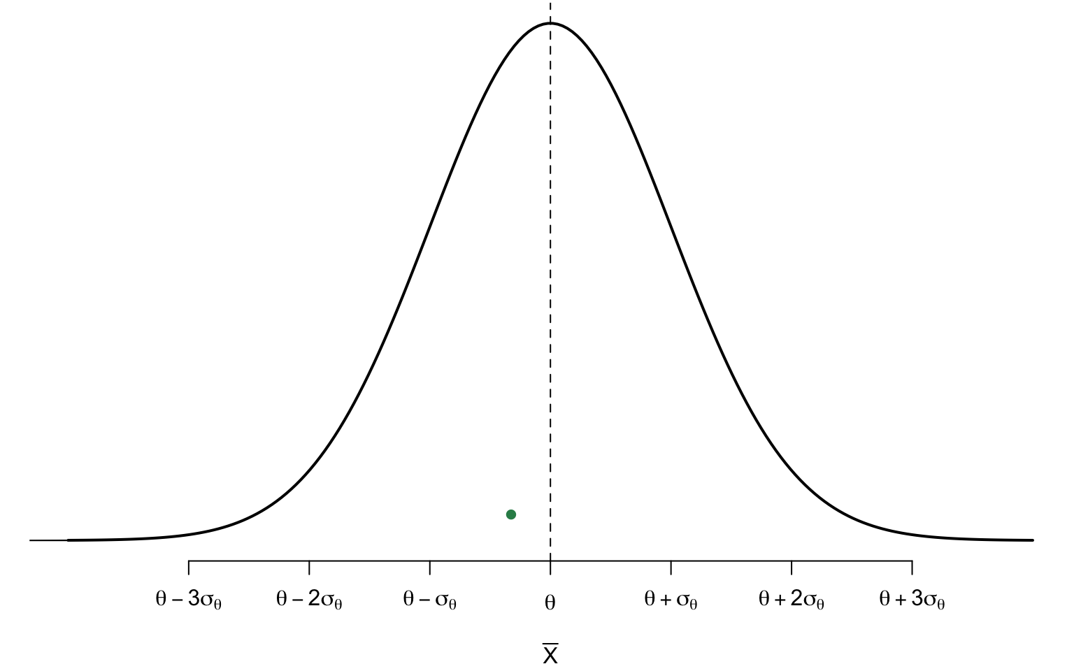
• Once the sample is observed, i.e. \(\overline{X} = \overline{x}\) and no longer a RV, the confidence interval becomes a fixed range of values.

• Since the parameter is also considered fixed, there is no more randomness associate with this interval and it either contains the true population parameter or it doesn’t.

Confidence

We use confidence rather than probability when describing CIs.

• e.g. we are 95 percent confident that the true population mean lies within \(1.96\cdot \frac{\sigma}{\sqrt{n}}\) of the observed sample mean.

Each row of points is a sample from the same normal distribution. The colored lines are 50% confidence intervals for the mean, μ. At the center of each interval is the sample mean, marked with a diamond. The blue intervals contain the population mean, and the red ones do not. [Source: wikipedia (Confidence interval, 2024)]

Comments

• When \(\overline{X}\) is still a random variable, we can interpret a confidence interval in terms of probability.

• The confidence level (e.g., 95%) represents the probability that the interval, if constructed repeatedly from different samples, will contain the true parameter.

• That is, if we were to collect many random samples and calculate the confidence interval for each sample, about 95% of those intervals would capture the true population mean \(\mu\).

• In this context, you can say that there is a 95% probability that a randomly chosen confidence interval will contain the true population mean.

100 95% CI based on 100 samples from a normal population with mean \(\mu\) and variance \(\sigma\). In theory 95% of them will contain the true value of μ. For this particular run, only 4 CI did not contain the true value of \(\mu\)

Example: SAT

95% Confidence Interval for the Population Mean

Suppose at a large high school, the seniors take the SAT exam. We draw a random sample of 10 of these students, and obtain their scores on the exam. These 10 students had a mean score of 1580. Construct a 95% confidence interval for the true mean SAT score of all seniors at this high school.

Important

Note: because this is a small sample size, before we take our CI we need to as ourselves if its reasonable to assuming a normal population.

Solution

Interpretation of CI

Assuming a normally distributed population and simple random sample from all senior SAT writers at this school, an interpretation of the interval is as follows:

✅ We can be 95% confident that the true mean SAT score of all senior writers at this school lies between 1431 and 1729.

Wrong interpretations

❌ We can be 95% confidence that the true mean SAT score of 10 sampled students, falls within the range of 1431 to 1729.

Important

It’s essential to note that the confidence interval pertains to a population parameter (here \(\mu\)), not a statistic (\(\bar {X}\)).

Wrong interpretations

❌ 95% of senior SAT writers at this school have SAT scores that lie between 1431 and 1729.

• implies a level of certainty about individual scores, confidence interval for the mean does not inform us about the proportion of the population that lies withinthe interval.

A confidence interval is about the range of likely values for a population parameter, not for individuals.

Balka for second pt: This is wrong, since a confidence interval for the mean does not inform us about the proportion of the population that lies withinthe interval. It is conceivable that 0% of the population lies within the 95% confidence interval for the mean.)

Recall

Sampling distribution for sample proportions

When observations are independent and the sample size is sufficiently large¹, the sample proportion \(\hat p\) is given by

\[ \hat p = \frac{X_1 + X_2 + \dots X_n}{n} \rightarrow N\left(\mu_{\hat p} = p, SE_{\hat p} = \sqrt{\frac{p(1-p)}{n}}\right) \]

we’ll estimate the SE by plugging in our estimate

1. when \(np \geq 10\) and \(n(1-p) \geq 10\)

General CI Construction

Where \(\frac{(\hat{\theta} - \theta)}{SE_{\hat \theta}} \sim N(0,1)\) and for a given \(\alpha, (0 <\alpha<1)\):

\[ \begin{align*} P \left( -z^* < \frac{(\hat{\theta} - \theta)}{SE_{\hat \theta}} < z^* \right) = 1-\alpha\\ P \left( -z^*SE < \hat{\theta} -\theta < z^* SE\right) = 1-\alpha\\ P \left( z^* SE > \theta - \hat{\theta} > - z^*SE \right) = 1-\alpha\\ P \left(\hat{\theta} -z^*SE < \theta < \hat{\theta} + z^* SE\right) = 1-\alpha\\ \end{align*} \]

where \(z^* = P(Z>\alpha/2)\) (or \(z_{\alpha/2}\)) for \(Z\sim N(0,1)\).

Notation

• The confidence level is given by \(C = 1-\alpha\)

  • e.g. when \(\alpha = 0.02\), our confidence level is 98%

• While a confidence level of 0.95 is quite standard, sometimes the problem will necessitate a higher level of confidence

• To find the \(z^*\) value that satisfies this formula, we could either use standard normal tables or software like R.

95% confidence is standard, though some situations call for a much more narrow CI, such as astrophysics or nuclear weapons.

1. \(\alpha\) is the so-called significance level; it will play a primary role with hypothesis testing
2. To emphasize that \(z^*\) (sometimes called the “z-critical value” or “z-score”) relies on \(\alpha\) you may alternatively see it be written as, \(z_\alpha\) or \(z_{\alpha/2}\).

\(100(C)\%\) Confidence Interval for a Population Proportion

Let \(X_1, \dots, X_n\) be a random sample from a population where each observation is binary (success/failure). A \(100(C)\%\) confidence interval for the population proportion \(p\) is given in the form:

\[\hat{p} \pm m \quad \text{or} \quad (\hat{p} - m, \hat{p} + m)\]

• where \(m\) is called the margin of error, given by:

  \[m = z^* \times \sqrt{\frac{\hat{p}(1 - \hat{p})}{n}}\]

• \(z^*\) is the critical value from the standard normal distribution such that:

  \[P(-z^* < Z < z^*) = C\]

  where \(C\) is the confidence level and \(n\) is the sample size.

A confidence interval (CI) for a population proportion provides a range of plausible values for the true population proportion \(p\) based on a sample proportion \(\hat{p}\). It quantifies the uncertainty in estimating \(p\) from sample data.

The general form of a confidence interval for a proportion is: \[ \hat p \pm 1.96 \sqrt{\frac{p(1-p)}{n}} \]

A 95% confidence interval for \(\hat p\) would therefore be given by:

\[ \hat p \pm 1.96 \sqrt{\frac{p(1-p)}{n}} \]

Assumptions for validity

The assumptions for CI are the same as that for the sampling distribution of \(\hat p\)

1. Random Sampling: The sample must be representative of the population.
2. Normal Approximation: The sample size should be large enough for the normal approximation to hold, which typically requires: \(n\hat p \geq 10\) and \(n(1-\hat p) \geq 10\)

ChatGPT example

Exercise: Use of ChatGPT

In a November 2023 research survey conducted by Pew Research about 13% of all U.S. teens have used the generative artificial intelligence (AI) chatbot in their schoolwork. This survey was conducted online from Sept. 26 to Oct. 23, 2023 and sampled 1,453 U.S. teens ages 13 to 17 who live with their parents by age, gender, race and ethnicity, household income, and other categories. Construct a 95% confidence interval for the population proportion based on this sample.

Solution

Margin of Error (m)

For the sample mean \(\overline{X}\),

\[ m = z^*\frac{\sigma}{\sqrt{n}} \]

For the sample proportion \(\hat{p}\),

\[ m = z^*\sqrt{\frac{p(1-p)}{n}} \]

The margin of error is a measure of the precision or uncertainty associated with the estimate derived from a sample. It is affected by \(n\) and \(z^*\).

• For the same confidence level \(1-\alpha\) as \(n\) increases the CI will get narrower
• For the same data as the confidence level \(1-\alpha\) increases the CI get wider

For \(\overline{X}\) as \(\sigma\) gets larger the CI get wider

For \(\hat p\), the narrowest CI is when \(p\) = 0.5

Width of CI

• The width of the CI (\(U - L\)) is a directly related to the margin of error (the smaller the better!)

• To accomplish this, the CI is constructed around the peak (center) of the sampling distribution such that \(\alpha/2\) appear in both tails.

• This ensures that we capture the most likely values while keeping the interval as narrow as possible.

• This is called a symmetric confidence intervals.

• While decreasing the value of \(z∗\) will also achieve a decrease in \(m\), doing so will decrease our confidence level.

Note that asymmetric confidence intervals exist, but they will necessarily be wider for normal models.

Asymmetric CI

Let’s calculate the width of a symmetric CI

alpha = 0.05
upper_z1 = qnorm(alpha/2, lower.tail = FALSE)
lower_z1 = qnorm(alpha/2)
(width1 = upper_z1 - lower_z1)

[1] 3.919928

Let’s calculate the width of a asymmetric CI

upper_z2 = qnorm(0.25*alpha, lower.tail = FALSE) # [1] 2.241403
lower_z2 = qnorm(0.75*alpha) # [1] -1.780464
(width2 = upper_z2 - lower_z2)

[1] 4.021867

Two 95% intervals on the standard normal distribution. The one shaded in blue extends from [-1.96, -1.96] and has a width of 3.92 one shaded in yellow extends from [-1.78,-1.78] and has a width of 4.02.

One-sided CI

As an extreme case, we might talk about one-sided CI, such that the entire \(\alpha\) probability is placed in either the lower or upper tail.

Example: Exclusive Relationships

A random sample of 50 college students were asked how many exclusive relationships they have been in so far. This sample yielded a mean of 3.2 and a standard deviation of 1.74. Estimate the true average number of exclusive relationships using this sample.

\[ \bar{x} = 3.2,\quad s = 1.74 \quad \text{and }n>30 \]

The approximate 95% confidence interval is defined as:

\[ \text{point estimate} \pm 1.96 \times SE \]

\[ \begin{align} SE = \sigma/\sqrt{n} = \frac{?}{\sqrt{n}} \end{align} \]

CI for unknown \(\sigma\)

You might be tempted to simply use \(s\) in place of \(\sigma\), HOWEVER,

\[ \dfrac{\bar{X} - \mu}{s/\sqrt{n}} \]

does NOT follow a standard normal distribution!

Estimating \(\sigma\) by \(s\) adds some more uncertainty and thus greater variability.

Unknown \(\sigma\)

Student-\(t\) Statistic

Let \(X_1, \dots, X_n\) be a sample from a normal population then,

\[ \dfrac{\bar{X} - \mu}{s/\sqrt{n}} \sim t_{\nu} \]

• where \(\nu = n-1\) is the degree’s of freedom for a student-\(t\) distribution

Reading the t-table

The \(t\)-table can be downloaded here

• rows = the degrees of freedom

• col = right-tail probabilities

• body cell values = t-values

Ttable Example 1

Examples:

\[ \begin{align} \Pr(t_8 > 1.397) &= 0.10 \end{align} \]

Ttable Example 2

Example:

\[ \Pr(t_5 > 4.5) < 0.005 \]

Assumptions for validity

When the sample is not drawn from a normal distribution, this result is approximate (thanks to the CLT) under certain conditions:

1. Independence: The observations in the sample must be independent.
2. Sample Size: The sample size should be reasonably large.

This is a result of the Central Limit Theorem, which states that the distribution of the sample mean becomes approximately normal as the sample size increases, regardless of the shape of the population distribution.

The key conditions for the validity of using the t-distribution are:

While there is no strict rule, a sample size of around 30 or more is often considered sufficient for the Central Limit Theorem to apply. However, the larger the sample size, the better the approximation.

CI for \(\mu\) (\(\sigma\) unknown)

100(C) Confidence Interval (unknown \(\sigma\))

Let \(X_1, \dots, X_n\) be a sample from a normal population then a \(100(C)\)% confidence interval for \(\mu\) is given in the form

\[ \begin{align} \bar{x} \ \pm m \quad\quad\text{ or} \\ (\bar{x} - m , \bar{x} + m) \end{align} \]

• where \(m\) is called the margin of error given by \(t^* + s/\sqrt{n}\)

• \(t^*\) is the value such that \(P(-t^* < t_{\nu} < t^*) = C\) where \(\nu = n-1\) and \(n\) is the sample size.

Conditions for using \(t\)

Conditions for using the t-distribution

The conditions for using the t-distribution are as follows:

1. Random Sampling: The data should be collected through a process of random sampling or a process that mimics random sampling.

2. Independence: The observations in the sample must be independent of each other.

3. Approximate Normality or Sufficiently Large Sample: While the t-distribution is robust to deviations from normality, it works best when the sample size is reasonably large (typically \(n \geq 30\) ).

Note: If the sample size is small and the population distribution is heavily skewed or has heavy tails, using the t-distribution might not be appropriate.

Returning to our example…

Example: Exclusive Relationships

A random sample of 50 college students were asked how many exclusive relationships they have been in so far. This sample yielded a mean of 3.2 and a standard deviation of 1.74. Estimate the true average number of exclusive relationships using this sample.

\[ \bar{x} = 3.2,\quad s = 1.74 \quad \text{and }n>30 \]

The approximate 95% confidence interval is defined as:

\[ \text{point estimate} \pm t^* \frac{s}{\sqrt{n}} \]

\[ \begin{align} SE = \frac{s}{\sqrt{n}} = \frac{1.74}{\sqrt{50}} = 0.2460732 \end{align} \]

\(t^*\) = -2.0095752

\[ \begin{align} \bar{x} \pm 2 \times SE & \rightarrow 3.2 \pm 2 \times 0.25 \\ & \rightarrow (3.2 - 0.5, 3.2 + 0.5) \\ & \rightarrow (2.7, 3.7) \end{align} \]

3.2 + c(1,-1)*qt(0.025, 50-1)*1.74/sqrt(50)

[1] 2.705497 3.694503

\(t^*\) using the tables

Since 50 is not on our table, we round down to the nearest integer (in this case 38).

We need to find the \(t^*\) that satisfies:

\[ \begin{align} \Pr(t_{50} > ?) &= 0.05\\ \implies ? &\approx 2.024 \end{align} \]

Important

Always round down¹ to the nearest available df in the table to ensure the confidence level is at least as high as desired. Rounding up may underestimate the critical value, leading to a less conservative interval.

qt(0.05/2, df = 50-1, lower.tail = FALSE)

[1] 2.009575

1. Note that is will be more conservative than that produced in R.

\(t^*\) using R

pt(q, df, ncp, lower.tail = TRUE)
qt(p, df, ncp, lower.tail = TRUE)

Argument	Description
x, q	vector of quantiles.
p	vector of probabilities.
df	degrees of freedom (>0>0, maybe non-integer). df = Inf is allowed.

\(t^*\) Comparison

Using the tables with conservative \(\nu\) = 38:

\[ \begin{align} \Pr(t_{50} > t^*) &= 0.05\\ \implies t^* &\approx 1.96\\ [2.6577&,3.7423]\\ \text{Width} &= 1.0846 \end{align} \]

Using R with the \(\nu = 50-1 = 49\)

\[ \begin{align} t^* &= 2.0095752 \\ [2.7055&,3.6945]\\ \text{Width} &= 0.989 \end{align} \]

qt(0.05/2, df = 50-1, lower.tail = FALSE)

[1] 2.009575

\(t^*\) Comparison

If we incorrectly round up (to \(\infty\)) \[ \begin{align} \Pr(t_{50} > t^*) &= 0.05\\ \implies t^* &\approx 1.96\\ [2.7177&,3.6823]\\ \text{Width} &= 0.9646 \end{align} \]

Using R with the \(\nu = 50-1 = 49\)

\[ \begin{align} t^* &= 2.0095752 \\ [2.7055&,3.6945]\\ \text{Width} &= 0.989 \end{align} \]

qt(0.05/2, df = 50-1, lower.tail = FALSE)

[1] 2.009575

iClicker

Interpretation of Confidence intervals

Which of the following is the correct interpretation of this confidence interval. We are 95% confident that…

1. the average number of exclusive relationships college students in this sample have been in is between 2.7 and 3.7.
2. college students on average have been in between 2.7 and 3.7 exclusive relationships.
3. a randomly chosen college student has been in 2.7 to 3.7 exclusive relationships.
4. 95% of college students have been in 2.7 to 3.7 exclusive relationships.

Example:

Example: fecundity

A study investigated per diem fecundity (number of eggs laidper female per day for the first 14 days of life) for a strain of Drosophila melanogaster. Per diem fecundity was measured for 25 females, and the results are listed below. Calculate the appropriate 95% CI.

data = c(14.9, 19.3, 20.3, 22.6, 23.4,
27.4, 28.2, 29.2, 29.5, 30.4,
33.7, 33.8, 34.4, 35.4, 36.6,
36.9, 37.3, 37.6, 37.9, 40.4,
41.7, 41.8, 42.4, 47.4, 51.8)

\(n\) = length(data) = 25

\(\bar{x}\) = mean(data) = 33.372

\(s\) = sd(data) = 8.9420132

Data Plotted

boxplot(data); hist(data); qqnorm(data);qqline(data)

Plot to assess the normality of the data before calculating the confidence interval. This is necessary to determine whether using a t-distribution for constructing the confidence interval is appropriate.

The boxplot and normal quantile-quantile plot show no major violations of the normality assumptio

QQplot

• A QQ plot, or Quantile-Quantile plot, is a graphical tool used to assess whether a dataset follows a particular theoretical distribution, often the normal distribution. It compares the quantiles of the observed data to the quantiles of a specified theoretical distribution.

• For a normal distribution, the QQ plot would ideally show points forming a straight line along the line of equality. Deviations from the line suggest departures from normality.

Balka pg 209 (bottom)

The sample size is 25, which yields \((n - 1 = 25 - 1 = 24)\) degrees of freedom.

From the table or software, we can find that \(t_{24}(0.025) = 2.064\).

The standard error is

Putting these values into the confidence interval formula: \[ \begin{align} &\bar{X} \pm t^* \cdot SE(\bar{X}) \\ &= 33.372 \pm 2.064 \times 1.788 \\ &= 33.372 \pm 3.691 \end{align} \] Which works out to approximately (29.7, 37.1).

The sample size is 25, which yields \((n - 1 = 25 - 1 = 24)\) degrees of freedom. From the table or software, we can find that \(t_{24}(0.025) = 2.064\) The standard error is \[ \hat \sigma_{\bar{X}} = \frac{s}{\sqrt{n}} = \frac{8.9420132}{\sqrt{25}} = 1.7884026 \approx 1.788 \]

Putting these values into the confidence interval formula: \[ \begin{align} &\bar{X} \pm t^*\cdot SE(\bar{X}) \\ &= 33.372 \pm 2.064 \times 1.788 \\ &= 33.372 \pm 3.691 \end{align} \] Which works out to approximately (29.7, 37.1).