Lecture 5: Likelihood and Parameter Estimation

STAT 205: Introduction to Mathematical Statistics

Dr. Irene Vrbik

University of British Columbia Okanagan

Outline

In this lecture we will be covering:

Introduction

  • Many applied statistical analysis problems involves estimating population parameters

    • e.g. mean \(\mu\), proportion \(p\), variance \(\sigma^2\)
  • Direct observation of these numerical characteristics may not be possible, so random variables are observed

    • e.g. sample mean/proportion/variance \(\overline{X}\)/\(\hat p\)/\(S^2\)

Objective: Develop methods using sample data (random variables) to gain information about unknown population characteristics.

Simple Random Samples

Population

πŸ§πŸ§πŸ»πŸ§πŸ½πŸ§πŸΎπŸ§πŸΏπŸ§β€β™€οΈπŸ§πŸ»β€β™€οΈπŸ§πŸΌβ€β™€οΈπŸ§πŸ½β€β™€οΈπŸ§πŸΎβ€β™€οΈπŸ§πŸΏβ€β™€οΈπŸ§β€β™‚οΈ

πŸ§β€β™‚οΈπŸ§πŸ½β€β™‚οΈπŸ§πŸΎβ€β™‚οΈπŸ§πŸΏβ€β™‚οΈπŸ§πŸΎβ€β™€οΈπŸ§πŸΏβ€β™€οΈπŸ§πŸ½β€β™‚οΈπŸ§πŸΏπŸ§β€β™‚οΈπŸ§πŸ½β€β™‚οΈπŸ§πŸΏπŸ§πŸΌβ€β™€οΈ

πŸ§πŸΏβ€β™‚οΈπŸ§πŸ§πŸ»πŸ§β€β™‚οΈπŸ§πŸ½πŸ§πŸΎπŸ§πŸΎβ€β™‚οΈπŸ§β€β™€οΈπŸ§πŸ»β€β™€οΈπŸ§πŸΌβ€β™€οΈπŸ§πŸ½β€β™€οΈπŸ§β€β™‚οΈ

πŸ§πŸΏβ€β™€οΈπŸ§πŸ§πŸ»πŸ§β€β™‚οΈπŸ§πŸ½πŸ§πŸΏβ€β™‚οΈπŸ§πŸΎπŸ§πŸΎβ€β™€οΈπŸ§πŸΎβ€β™‚οΈπŸ§β€β™€οΈπŸ§πŸ»β€β™€οΈπŸ§πŸ½β€β™€οΈ

Important

Taking an SRS minimizes bias, enables valid statistical inferences, and makes results generalizable.

\[\downarrow\]

Sample

πŸ§πŸ§πŸΎπŸ§πŸΌβ€β™€οΈπŸ§πŸ½β€β™€οΈπŸ§β€β™‚οΈπŸ§πŸ½β€β™‚οΈ

SRS (Simple Random Sample)

A Simple Random Sample (SRS) is a sampling method in which every element in the population has an equal probability of being selected, and each subset of the population of a given size has an equal chance of being chosen.

Population Distribution and Parameter Estimation

  • We begin with a simple random sample of size \(n\) from a population.

  • Parameters of interest are unknown but assumed to follow a known distribution.

  • Estimation focuses on obtaining the best possible estimates of population parameters.

Example: Normal Population

Population

πŸ§πŸ§πŸ»πŸ§πŸ½πŸ§πŸΎπŸ§πŸΏπŸ§β€β™€οΈπŸ§πŸ»β€β™€οΈπŸ§πŸΌβ€β™€οΈπŸ§πŸ½β€β™€οΈπŸ§πŸΎβ€β™€οΈπŸ§πŸΏβ€β™€οΈπŸ§β€β™‚οΈ

πŸ§β€β™‚οΈπŸ§πŸ½β€β™‚οΈπŸ§πŸΎβ€β™‚οΈπŸ§πŸΏβ€β™‚οΈπŸ§πŸΎβ€β™€οΈπŸ§πŸΏβ€β™€οΈπŸ§πŸ½β€β™‚οΈπŸ§πŸΏπŸ§β€β™‚οΈπŸ§πŸ½β€β™‚οΈπŸ§πŸΏπŸ§πŸΌβ€β™€οΈ

πŸ§πŸΏβ€β™‚οΈπŸ§πŸ§πŸ»πŸ§β€β™‚οΈπŸ§πŸ½πŸ§πŸΎπŸ§πŸΎβ€β™‚οΈπŸ§β€β™€οΈπŸ§πŸ»β€β™€οΈπŸ§πŸΌβ€β™€οΈπŸ§πŸ½β€β™€οΈπŸ§β€β™‚οΈ

πŸ§πŸΏβ€β™€οΈπŸ§πŸ§πŸ»πŸ§β€β™‚οΈπŸ§πŸ½πŸ§πŸΏβ€β™‚οΈπŸ§πŸΎπŸ§πŸΎβ€β™€οΈπŸ§πŸΎβ€β™‚οΈπŸ§β€β™€οΈπŸ§πŸ»β€β™€οΈπŸ§πŸ½β€β™€οΈ

\[\downarrow \text{SRS}\]

Sample

πŸ§πŸ§πŸΎπŸ§πŸΌβ€β™€οΈπŸ§πŸ½β€β™€οΈπŸ§β€β™‚οΈπŸ§πŸ½β€β™‚οΈ

Population Distribution

\[ \begin{align} & f(x;\mu, \sigma) \end{align} \]

Population Parameters

\[ \begin{align} \mu &= ? & \sigma^2 &= ? \end{align} \]

Example: Exponential Distribution

Population

πŸ§πŸ§πŸ»πŸ§πŸ½πŸ§πŸΎπŸ§πŸΏπŸ§β€β™€οΈπŸ§πŸ»β€β™€οΈπŸ§πŸΌβ€β™€οΈπŸ§πŸ½β€β™€οΈπŸ§πŸΎβ€β™€οΈπŸ§πŸΏβ€β™€οΈπŸ§β€β™‚οΈ

πŸ§β€β™‚οΈπŸ§πŸ½β€β™‚οΈπŸ§πŸΎβ€β™‚οΈπŸ§πŸΏβ€β™‚οΈπŸ§πŸΎβ€β™€οΈπŸ§πŸΏβ€β™€οΈπŸ§πŸ½β€β™‚οΈπŸ§πŸΏπŸ§β€β™‚οΈπŸ§πŸ½β€β™‚οΈπŸ§πŸΏπŸ§πŸΌβ€β™€οΈ

πŸ§πŸΏβ€β™‚οΈπŸ§πŸ§πŸ»πŸ§β€β™‚οΈπŸ§πŸ½πŸ§πŸΎπŸ§πŸΎβ€β™‚οΈπŸ§β€β™€οΈπŸ§πŸ»β€β™€οΈπŸ§πŸΌβ€β™€οΈπŸ§πŸ½β€β™€οΈπŸ§β€β™‚οΈ

πŸ§πŸΏβ€β™€οΈπŸ§πŸ§πŸ»πŸ§β€β™‚οΈπŸ§πŸ½πŸ§πŸΏβ€β™‚οΈπŸ§πŸΎπŸ§πŸΎβ€β™€οΈπŸ§πŸΎβ€β™‚οΈπŸ§β€β™€οΈπŸ§πŸ»β€β™€οΈπŸ§πŸ½β€β™€οΈ

\[\downarrow \text{SRS}\]

Sample

πŸ§πŸ§πŸΎπŸ§πŸΌβ€β™€οΈπŸ§πŸ½β€β™€οΈπŸ§β€β™‚οΈπŸ§πŸ½β€β™‚οΈ

Population Distribution

\[ \begin{align} & f(x; \lambda) = \lambda e^{-\lambda x} & x \geq 0 \end{align} \]

Population Parameters

\[ \begin{align} \lambda &= ? \end{align} \]

Example: Beta Distribution

Population

πŸ§πŸ§πŸ»πŸ§πŸ½πŸ§πŸΎπŸ§πŸΏπŸ§β€β™€οΈπŸ§πŸ»β€β™€οΈπŸ§πŸΌβ€β™€οΈπŸ§πŸ½β€β™€οΈπŸ§πŸΎβ€β™€οΈπŸ§πŸΏβ€β™€οΈπŸ§β€β™‚οΈ

πŸ§β€β™‚οΈπŸ§πŸ½β€β™‚οΈπŸ§πŸΎβ€β™‚οΈπŸ§πŸΏβ€β™‚οΈπŸ§πŸΎβ€β™€οΈπŸ§πŸΏβ€β™€οΈπŸ§πŸ½β€β™‚οΈπŸ§πŸΏπŸ§β€β™‚οΈπŸ§πŸ½β€β™‚οΈπŸ§πŸΏπŸ§πŸΌβ€β™€οΈ

πŸ§πŸΏβ€β™‚οΈπŸ§πŸ§πŸ»πŸ§β€β™‚οΈπŸ§πŸ½πŸ§πŸΎπŸ§πŸΎβ€β™‚οΈπŸ§β€β™€οΈπŸ§πŸ»β€β™€οΈπŸ§πŸΌβ€β™€οΈπŸ§πŸ½β€β™€οΈπŸ§β€β™‚οΈ

πŸ§πŸΏβ€β™€οΈπŸ§πŸ§πŸ»πŸ§β€β™‚οΈπŸ§πŸ½πŸ§πŸΏβ€β™‚οΈπŸ§πŸΎπŸ§πŸΎβ€β™€οΈπŸ§πŸΎβ€β™‚οΈπŸ§β€β™€οΈπŸ§πŸ»β€β™€οΈπŸ§πŸ½β€β™€οΈ

\[\downarrow \text{SRS}\]

Sample

πŸ§πŸ§πŸΎπŸ§πŸΌβ€β™€οΈπŸ§πŸ½β€β™€οΈπŸ§β€β™‚οΈπŸ§πŸ½β€β™‚οΈ

Population Distribution

\[ \begin{align} f(x; \alpha, \beta) = \begin{cases} \frac{x^{\alpha - 1}(1 - x)^{\beta - 1}}{\text{B}(\alpha, \beta)} & 0 \leq x \leq 1, \\ 0 & \text{o.w} \end{cases} \end{align} \]

Population Parameters

\[ \begin{align} \alpha = ? && \beta &= ? \end{align} \]

More Generally

Population

πŸ§πŸ§πŸ»πŸ§πŸ½πŸ§πŸΎπŸ§πŸΏπŸ§β€β™€οΈπŸ§πŸ»β€β™€οΈπŸ§πŸΌβ€β™€οΈπŸ§πŸ½β€β™€οΈπŸ§πŸΎβ€β™€οΈπŸ§πŸΏβ€β™€οΈπŸ§β€β™‚οΈ

πŸ§β€β™‚οΈπŸ§πŸ½β€β™‚οΈπŸ§πŸΎβ€β™‚οΈπŸ§πŸΏβ€β™‚οΈπŸ§πŸΎβ€β™€οΈπŸ§πŸΏβ€β™€οΈπŸ§πŸ½β€β™‚οΈπŸ§πŸΏπŸ§β€β™‚οΈπŸ§πŸ½β€β™‚οΈπŸ§πŸΏπŸ§πŸΌβ€β™€οΈ

πŸ§πŸΏβ€β™‚οΈπŸ§πŸ§πŸ»πŸ§β€β™‚οΈπŸ§πŸ½πŸ§πŸΎπŸ§πŸΎβ€β™‚οΈπŸ§β€β™€οΈπŸ§πŸ»β€β™€οΈπŸ§πŸΌβ€β™€οΈπŸ§πŸ½β€β™€οΈπŸ§β€β™‚οΈ

πŸ§πŸΏβ€β™€οΈπŸ§πŸ§πŸ»πŸ§β€β™‚οΈπŸ§πŸ½πŸ§πŸΏβ€β™‚οΈπŸ§πŸΎπŸ§πŸΎβ€β™€οΈπŸ§πŸΎβ€β™‚οΈπŸ§β€β™€οΈπŸ§πŸ»β€β™€οΈπŸ§πŸ½β€β™€οΈ

\[\downarrow \text{SRS}\]

Sample

πŸ§πŸ§πŸΎπŸ§πŸΌβ€β™€οΈπŸ§πŸ½β€β™€οΈπŸ§β€β™‚οΈπŸ§πŸ½β€β™‚οΈ

Population Distribution

\[ \begin{align} f(x; \theta_1, \dots, \theta_l) \end{align} \]

Population Parameters

\[ \begin{align} \theta_1 = ? \quad \theta_2 &= ? \quad \dots \quad \theta_l = ? \end{align} \]

Population Assumption

Assume the population follows some distribution with parameters \(\theta_1\), through \(\theta_l\) to be estimated.

Types of Estimators

Two types of estimators:

  • Point estimators provide a single β€œbest guess” for the parameter.
  • Interval estimators, also known as a confidence interval, provides a range of values within which the true value of the parameter is expected to fall, along with a level of confidence.

Setup

Sampling Assumptions

Let \(X = (X_1, \dots, X_n)\) be independent and identically distributed (i.i.d) random variables (RVs) with a probability density function (pdf) or probability mass function (pmf) \(f(x; \theta_1, \dots, \theta_l)\), where \(\theta_1, \dots, \theta_l\) are the unknown population parameters.

RIS (Random Independent Sample)

A Random Independent Sample (RIS) of size \(n\) involves a sampling method where individuals are chosen randomly and independently from the population.

Notation

Estimator

An estimator, \(\hat \Theta(X_1, X_2, \dots, X_n)\) is a rule, formula, or function used to calculate an estimate based on sample data. We will denote the estimator by \(\hat \Theta\) (captital theta) to emphasize that it representing a random variable that depends on the random sample.

Point Estimate

A point estimate, (or simply, estimate) \(\hat \theta(x_1, x_2, \dots, x_n)\) is the numerical value produced by applying the estimator to a specific sample. It is the realized value of the estimator after data collection. It is typically written simply as \(\hat \theta\).

Normal Population

Population

πŸ§πŸ§πŸ»πŸ§πŸ½πŸ§πŸΎπŸ§πŸΏπŸ§β€β™€οΈπŸ§πŸ»β€β™€οΈπŸ§πŸΌβ€β™€οΈπŸ§πŸ½β€β™€οΈπŸ§πŸΎβ€β™€οΈπŸ§πŸΏβ€β™€οΈπŸ§β€β™‚οΈ

πŸ§β€β™‚οΈπŸ§πŸ½β€β™‚οΈπŸ§πŸΎβ€β™‚οΈπŸ§πŸΏβ€β™‚οΈπŸ§πŸΎβ€β™€οΈπŸ§πŸΏβ€β™€οΈπŸ§πŸ½β€β™‚οΈπŸ§πŸΏπŸ§β€β™‚οΈπŸ§πŸ½β€β™‚οΈπŸ§πŸΏπŸ§πŸΌβ€β™€οΈ

πŸ§πŸΏβ€β™‚οΈπŸ§πŸ§πŸ»πŸ§β€β™‚οΈπŸ§πŸ½πŸ§πŸΎπŸ§πŸΎβ€β™‚οΈπŸ§β€β™€οΈπŸ§πŸ»β€β™€οΈπŸ§πŸΌβ€β™€οΈπŸ§πŸ½β€β™€οΈπŸ§β€β™‚οΈ

πŸ§πŸΏβ€β™€οΈπŸ§πŸ§πŸ»πŸ§β€β™‚οΈπŸ§πŸ½πŸ§πŸΏβ€β™‚οΈπŸ§πŸΎπŸ§πŸΎβ€β™€οΈπŸ§πŸΎβ€β™‚οΈπŸ§β€β™€οΈπŸ§πŸ»β€β™€οΈπŸ§πŸ½β€β™€οΈ

\[\downarrow \text{RIS}\]

Sample

πŸ§πŸ§πŸΎπŸ§πŸΌβ€β™€οΈπŸ§πŸ½β€β™€οΈπŸ§β€β™‚οΈπŸ§πŸ½β€β™‚οΈ

Population Distribution

\[ \begin{align} & f(x;\mu, \sigma) \end{align} \]

Sample Statistic (RV)

\[ \hat \mu = \frac{X_1 + \dots + X_n}{n} \]

the sample mean function is our estimator (RV) of the population parameter \(\mu\).

Normal Population

Population

πŸ§πŸ§πŸ»πŸ§πŸ½πŸ§πŸΎπŸ§πŸΏπŸ§β€β™€οΈπŸ§πŸ»β€β™€οΈπŸ§πŸΌβ€β™€οΈπŸ§πŸ½β€β™€οΈπŸ§πŸΎβ€β™€οΈπŸ§πŸΏβ€β™€οΈπŸ§β€β™‚οΈ

πŸ§β€β™‚οΈπŸ§πŸ½β€β™‚οΈπŸ§πŸΎβ€β™‚οΈπŸ§πŸΏβ€β™‚οΈπŸ§πŸΎβ€β™€οΈπŸ§πŸΏβ€β™€οΈπŸ§πŸ½β€β™‚οΈπŸ§πŸΏπŸ§β€β™‚οΈπŸ§πŸ½β€β™‚οΈπŸ§πŸΏπŸ§πŸΌβ€β™€οΈ

πŸ§πŸΏβ€β™‚οΈπŸ§πŸ§πŸ»πŸ§β€β™‚οΈπŸ§πŸ½πŸ§πŸΎπŸ§πŸΎβ€β™‚οΈπŸ§β€β™€οΈπŸ§πŸ»β€β™€οΈπŸ§πŸΌβ€β™€οΈπŸ§πŸ½β€β™€οΈπŸ§β€β™‚οΈ

πŸ§πŸΏβ€β™€οΈπŸ§πŸ§πŸ»πŸ§β€β™‚οΈπŸ§πŸ½πŸ§πŸΏβ€β™‚οΈπŸ§πŸΎπŸ§πŸΎβ€β™€οΈπŸ§πŸΎβ€β™‚οΈπŸ§β€β™€οΈπŸ§πŸ»β€β™€οΈπŸ§πŸ½β€β™€οΈ

\[\downarrow \text{RIS}\]

Sample

πŸ§πŸ§πŸΎπŸ§πŸΌβ€β™€οΈπŸ§πŸ½β€β™€οΈπŸ§β€β™‚οΈπŸ§πŸ½β€β™‚οΈ

Population Distribution \[ \begin{align} & f(x;\mu, \sigma) \end{align} \]

Point Estimate

\[ \begin{align} {\hat \mu} &= \frac{x_1 + \dots + x_n}{n} \\ &= \frac{170 + 192 + \dots + 155}{6} \\ &= 167.7 \end{align} \]

the value, 167.7, is the estimate of the population parameter \(\mu\).

More Generally

Population

πŸ§πŸ§πŸ»πŸ§πŸ½πŸ§πŸΎπŸ§πŸΏπŸ§β€β™€οΈπŸ§πŸ»β€β™€οΈπŸ§πŸΌβ€β™€οΈπŸ§πŸ½β€β™€οΈπŸ§πŸΎβ€β™€οΈπŸ§πŸΏβ€β™€οΈπŸ§β€β™‚οΈ

πŸ§β€β™‚οΈπŸ§πŸ½β€β™‚οΈπŸ§πŸΎβ€β™‚οΈπŸ§πŸΏβ€β™‚οΈπŸ§πŸΎβ€β™€οΈπŸ§πŸΏβ€β™€οΈπŸ§πŸ½β€β™‚οΈπŸ§πŸΏπŸ§β€β™‚οΈπŸ§πŸ½β€β™‚οΈπŸ§πŸΏπŸ§πŸΌβ€β™€οΈ

πŸ§πŸΏβ€β™‚οΈπŸ§πŸ§πŸ»πŸ§β€β™‚οΈπŸ§πŸ½πŸ§πŸΎπŸ§πŸΎβ€β™‚οΈπŸ§β€β™€οΈπŸ§πŸ»β€β™€οΈπŸ§πŸΌβ€β™€οΈπŸ§πŸ½β€β™€οΈπŸ§β€β™‚οΈ

πŸ§πŸΏβ€β™€οΈπŸ§πŸ§πŸ»πŸ§β€β™‚οΈπŸ§πŸ½πŸ§πŸΏβ€β™‚οΈπŸ§πŸΎπŸ§πŸΎβ€β™€οΈπŸ§πŸΎβ€β™‚οΈπŸ§β€β™€οΈπŸ§πŸ»β€β™€οΈπŸ§πŸ½β€β™€οΈ

\[\downarrow \text{RIS}\]

Sample

πŸ§πŸ§πŸΎπŸ§πŸΌβ€β™€οΈπŸ§πŸ½β€β™€οΈπŸ§β€β™‚οΈπŸ§πŸ½β€β™‚οΈ

Population Distribution

\[ \begin{align} & f(x;\theta_1, \dots, \theta_l) \end{align} \]

Sample Statistic

\[ \hat \Theta = g(X_1, \dots, X_n) \]

Point Estimate

\[ \hat \theta = g(x_1, \dots, x_n) \]

Why the sample mean?

  • The sample mean is commonly used to estimate the population mean \(\mu\)

  • However we could have used other estimators:

    • the sample median
    • the mode
    • selected a height from our sample at random

Think-Pair-Share

πŸ€” What Makes a β€œgood” guess for \(\mu\)

Unbiased

To narrow down our choices, we will first insist that our estimators be unbiased meaning

\[ \mathbb{E}[\hat \Theta] = \theta \] or at least asymtotically unbiased, i.e.

\[ \mathbb{E}[\hat{\Theta}] \underset{n \to \infty}{\rightarrow} \theta \]

The difference \(\mathbb{E}[\hat \Theta] = \theta\) is called the bias of an estimator, and can be easily removed.

Unbiasedness Alone is Not Enough

  • An estimator being unbiased (or asymptotically unbiased) does not guarantee it is β€œgood.”

  • Example: Using \(\hat \Theta = X_1\) (the first observation) is an unbiased estimator for \(\mu\) but it wastes most of the sample information.

  • Thus being unbiased is only one essential ingredient of a good estimator, the other one is its variance (which we would like to keep as small as possible).

Consistency

A consistent estimator must have two properties:

  1. It must be asymtotically unbiased, \[ \mathbb{E}[\hat{\Theta}] \underset{n \to \infty}{\rightarrow} \theta \]
  2. Its variance must tend to zero with increasing sample size \[ \text{Var}[\hat{\Theta}] \underset{n \to \infty}{\rightarrow} 0 \]

MVUE

The Minimum Variance Unbiased Estimator (MVUE), \(\hat \Theta_{\text{MVUE}}\) satisfies the following two properties:

  1. The estimator is unbiased \(\mathbb{E}[\hat \Theta] = \theta\)

  2. Among all unbiased estimators of the parameter \(\theta\), the MVUE has the lowest variance. That is

    \[ \text{Var}(\hat \Theta_\text{MVUE}) \leq \text{Var}(\hat \Theta_\text{unbiased}) \] for any other unbiased estimator \(\hat \Theta_\text{unbiased}\)

Problem 1

The MVUE estimator may not exist.

  • The variance of an estimator is, in general, a function of \(\theta\)
  • Hence we compare functions of \(\theta\), not values.
  • Two unbiased estimators may have variances such that one is smaller in some range of \(\theta\) and bigger in another.
  • Neither estimator is then (uniformly) better than the other

Problem 2

  • How do we determine if the MVUE exists?

  • If we can determine that it exists, how do we find it?

  • We will return to these questions in a future lecture, but for now we should understand that practical challenges often lead statisticians to use alternative methods …

Methods of Finding Point Estimators

Two common ways of finding point estimators:

  • Method of Moments: sample moments are equated to their corresponding population moments to obtain estimates for the parameters.
  • Maximum likelihood estimation (MLE): seeks to find the values of model parameters that maximize the so-called likelihood function.

Method of Moments (MoM)

  • The method of moments is one of the oldest methods for estimating the parameters of a statistical model.

  • In this method, the population moments1 are equated to their sample counterparts, providing a set of equations that can be solved to obtain estimates for the parameters.

Population Moments

Theoretical/Population Moment

The \(k\)th (population) moment (about the origin) of a random variable \(X\), denoted \(\mu_k'\) is the expected value of \(X^k\). Hence \[ \mu_k' = \mathbb{E}[X^k] \]

E.g. the first moment (i.e. the mean) for select distributions:

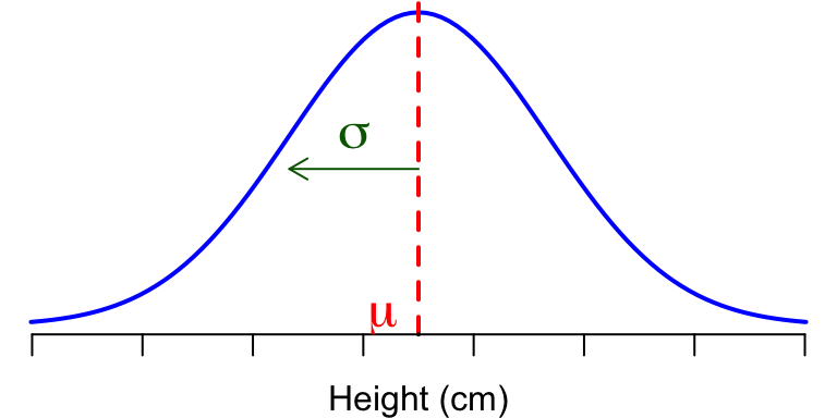
  • \(X\sim\) Normal\((\mu,\sigma)\) \(\mathbb{E}[X] = \mu\)
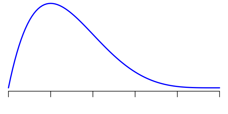
  • \(X\sim\) Exponential\((\lambda)\) \(\mathbb{E}[X] = \frac{1}{\lambda}\)
  • \(X\sim\) Beta\((\alpha,\beta)\) \(\mathbb{E}[X] = \frac{\alpha}{\alpha + \beta}\)

Note

Notice how \(\mathbb{E}[X]\) is a function of the parameters

Sample Moments

Sample moments are based on the sample data and provide empirical estimates of the unknown population moments.

Sample Moment

The \(k\)th sample moment (about the origin) \(m_k'\) is defined as the average of the \(k\)th powers of the observed data points. Hence

\[m_k' = \frac{1}{n} \sum_{i=1}^n X_i^k\]

Main Idea

Premise: \(m_k'\) should provide good estimates of the corresponding population moments \(\mu_k'\).

  • e.g. the sample mean (aka the first sample moment \(m'_1 = \frac{1}{n}\sum_{i=1}^n X_i\)) should provide a good guess for the population mean (aka the first population moment \(\mu_1' = \mathbb{E}[X^1]\)

  • similarly \(m'_2 = \frac{1}{n}\sum_{i=1}^n X_i^2\) provides a good guess for the second population moment \(\mu'_2 = \mathbb{E}[X^2]\)
MoM procedure (in words)

  1. Determine the number of parameters: First, identify how many parameters you need to estimate for your chosen distribution.
  2. Set up equations for moments: Set theoretical moments of the distribution (function of its parameters) equal to the corresponding sample moment (computed from the data)
  3. Solve for parameters: Solve the system of equations simultaneously to obtain estimates of the parameters. This often results in a system of equations that can be solved using algebraic or numerical methods.

MoM procedure

Suppose there are \(l\) parameters to be estimated, i.e. \(\theta = (\theta_1, \ldots, \theta_l)\).

  1. Find \(l\) population moments1, \(\mu_k'\), \(k = 1, 2, \ldots, l\).

  2. Find the corresponding \(l\) sample moments2, \(m_k'\), \(k = 1, 2, \ldots, l\)

  3. From the system of equations, \(\mu_k' = m_k'\), \(k = 1, 2, \ldots, l\), solve for the parameter \(\theta = (\theta_1, \ldots, \theta_l)\);
    this will be a moment estimator of \(\hat{\theta}\).

MoM: Normal Population

The Normal Distribution, \(f(x;\mu, \sigma)\), has two parameters: \(\mu\) and \(\sigma\). Hence we will need two sets of moments…

Population Moments

\[ \begin{align} \mu'_1 &= \mathbb{E}[X] = \mu\\ \mu'_2 &=\mathbb{E}[X^2]=\sigma^2 + \mu^2 \end{align} \]

Sample Moments

\[ \begin{align} m'_1 &= \frac{1}{n}\sum_{i=1}^n X_i \\ m'_2 &= \frac{1}{n}\sum_{i=1}^n X_i^2 \end{align} \]

Solving the system of Equations

Set the population moments equal to the sample moments and solve for the unknown parameters:

\[ \begin{align} \mu'_1 &=m'_1 \\ \mu &= \frac{1}{n}\sum_{i=1}^n X_i \\ \hat \mu &= \bar{X} \end{align} \]

\[ \begin{align} \mu'_2 &= m'_2\\ \sigma^2 + \mu^2 &= \frac{1}{n}\sum_{i=1}^n X_i^2\\ \sigma^2 &= \frac{1}{n}\sum_{i=1}^n X_i^2 - \mu^2\\ \implies \hat \sigma^2 &= \frac{1}{n}\sum_{i=1}^n X_i^2 - \bar{X}^2 \\ \end{align} \]

MoM: Exponential

The Exponential Distribution \(f(x;\lambda)\), has only one parameters: \(\lambda\). Hence we need one sets of moments…

Population Moments

\[ \begin{align} \mu'_1 &= \mathbb{E}[X] = \frac{1}{\lambda} \end{align} \]

Sample Moments

\[ \begin{align} m'_1 &= \frac{1}{n}\sum_{i=1}^n X_i \end{align} \]

Simple Algebra

Set the moments equal to each other and solve for the unknown parameter \(\lambda\):

\[ \begin{align} \mu'_1 & = m'_1 \\ \frac{1}{\lambda} &= \frac{1}{n}\sum_{i=1}^n X_i \\ \implies \lambda &= \frac{n}{\sum_{i=1}^n X_i} \end{align} \]

iClicker

Example: Bernoulli distribution

Let \(X_1, \dots, X_n\) be a random sample from a Bernoulli distribution with probability \(p\). Using the method of moments, find the estimator for \(p\).

  1. \(\hat p = \frac{\sum_{i=1}^nX_i}{n}\)
  2. \(\hat p = \frac{n}{\sum_{i=1}^nX_i}\)
  3. \(\hat p = \frac{\sum_{i=1}^nX_i^2}{n}\)
  4. \(\hat p = \frac{\mu }{n}\)
  5. None of the above

Solution

Comments

  • While intuitive and easy to apply, the method of moments usually does not yield β€œgood” estimators (they are not always efficient)

  • In some cases, the method of moments estimator may coincide with other well-known estimators, providing a unique solution.

  • However, in more complex models or under certain conditions, the method of moments may not produce a unique estimator.

Maximum Likelihood Estimation

The method of maximum likelihood estimation was proposed by Sir Ronald A. Fisher around 1922.
  • Maximum Likelihood Estimation (MLE) is a method for estimating the parameters of a statistical model.

  • The basic idea behind MLE is to find the values of the parameters that maximize the likelihood function, which measures how well the model explains the observed data.

Likelihood

Likelihood (definition)

Let \(f(x_1, \ldots, x_n; \theta)\), \(\theta \in \Theta \subseteq \mathbb{R}^k\), be the joint probability (or density) function of \(n\) random variables (\(X_1, \ldots, X_n\)) with sample values (\(x_1, \ldots, x_n\)). The likelihood function of the sample is given by: \[\begin{equation} L(\theta; x_1, \ldots, x_n) = f(x_1, \ldots, x_n; \theta) \end{equation}\] Note: \(L\) is a function of \(\theta\) for fixed sample values.

Likelihood Formula

If \((X_1, \ldots, X_n)\) are iid discrete random variables with probability mass function (PMF) \(p(x, \theta)\), then the likelihood function is given by: \[ \begin{align*} L(\theta) &= P(X_1 = x_1, \dots, X_n = x_n) \\ &= \prod_{i=1}^{n} P(X_i = x_i) \text{ by multiplication rule for independent RV}\\ &= \prod_{i=1}^{n} p(x_i; \theta) \end{align*} \]

And in the continuous case, if the density is \(f(x;\theta)\), then the likelihood function is: \[ L(\theta) = \prod_{i=1}^{n} f(x_i; \theta) \]

Comment about Likelihood

  • Although likelihood depends on the observed sample values \(x = (x_1, \ldots, x_n)\), is to be regarded as a function of the parameter \(\theta\).

  • In the discrete case, \(L(\theta; x_1, \ldots, x_n)\) gives the probability of observing \(x = (x_1, \ldots, x_n)\) for a given \(\theta\).

  • Thus, the likelihood function is a statistic, depending on the observed sample \(x = (x_1, \ldots, x_n)\).

Example: Normal Likelihood

Let \(X_1, \ldots, X_n\) be independent and identically distributed random variables following a normal distribution \(N(\mu, \sigma^2)\). Let \(x_1, \ldots, x_n\) be the corresponding sample values. Find the likelihood function.

Recall the pdf of Normal distribution:

\[\begin{equation} f(x; \mu, \sigma^2) = \frac{1}{\sqrt{2\pi\sigma^2}} \exp\left\{{-\frac{(x - \mu)^2}{2\sigma^2}}\right\} \end{equation}\]

Solution

MLEs

Maximum likelihood estimators (MLEs)

Maximum likelihood estimators or MLEs are those values of the parameters that maximize the likelihood function with respect to the parameter \(\theta\). That is, \[ \hat{\theta}_{\text{MLE}} = \underset{\theta \in \Theta}{\arg\max} \, L(\theta) \] where \(\Theta\) is the set of possible values of the parameter \(\theta\).

Calculus Comment

  • The maximum likelihood method typically involves maximizing a function of one or more variables.

  • Deriving maximum likelihood estimators (MLEs) generally involves some calculus

  • However, some situations may involve problem-specific techniques (see here for an example using Newton-Raphson method for the gamm distribution)

Procedure for finding the MLE

  1. Define the likelihood function, \(L(\theta)\).
  2. Often it is easier to take the natural logarithm (ln) of \(L(\theta)\).
  3. When applicable, differentiate \(\ln L(\theta)\) with respect to \(\theta\), and then equate the derivative to zero.
  4. Solve for the parameter \(\theta\), and we will obtain \(\hat{\theta}\).
  5. Check whether it is a maximizer or a global maximizer.

Example: MLE for geometric distribution

Suppose \(X_1, \ldots, X_n\) is a random sample from a geometric distribution with parameter \(p\), \(0 \leq p \leq 1\). Find the MLE.

Recall the probability mass function (PMF) of a geometric distribution with parameter \(p\), denoted as \(X \sim \text{Geometric}(p)\), is given by: \[ P(X = x) = p(1 - p)^{x-1} \quad \text{for } x = 1, 2, 3, \ldots \]

Solution

Plot the likelihood

The plotted likelihood for simulated data from a geometric distribution with \(p\) = 0.3.

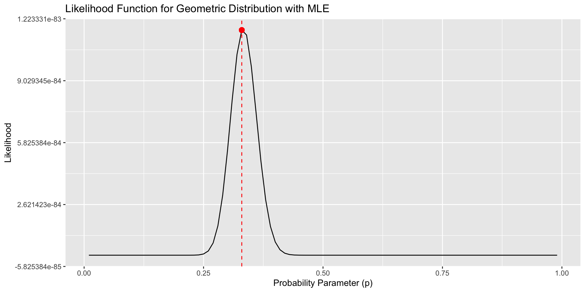
Plot the MLE

For this simulation the MLE is \(\hat p = 0.33\)

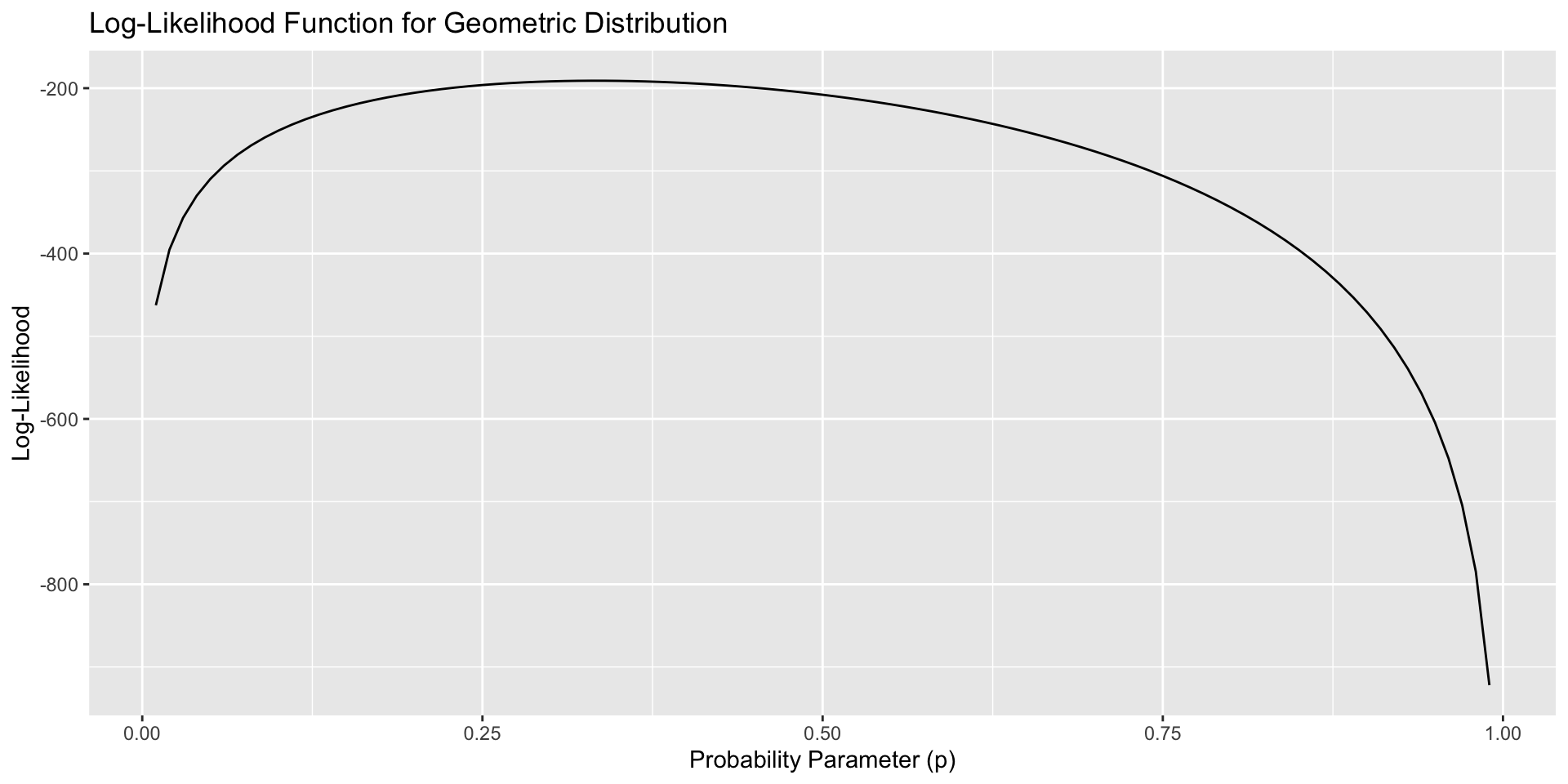
Plot the log-likelihood

The plotted log-likelihood for simulated data from a geometric distribution with \(p\) = 0.3.

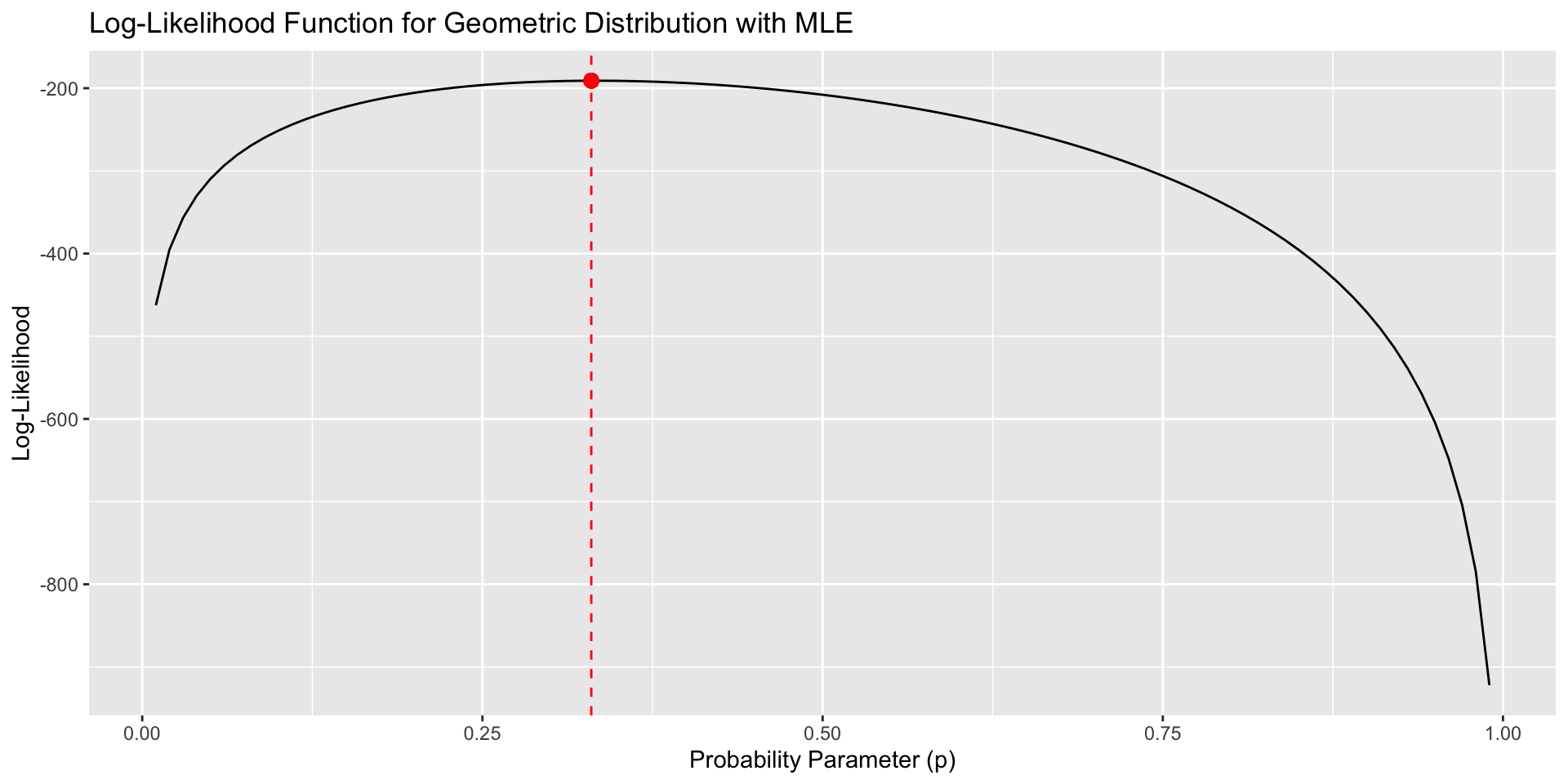
Plot the MLEs

Because the natural logarithm function is increasing, the maximum value of the likelihood function, if it exists, will occur at the same point as the maximum value of the log-likelihood function.

MLEs for multiple parameters

Let \((X_1, \ldots, X_n)\) be a random sample with joint probability mass function (if discrete) or probability density function (if continuous):

\[ L(\theta_1, \dots, \theta_m; x_1, \dots, x_n) = f(x_1, \ldots, x_n; \theta_1, \ldots, \theta_m) \]

where the values of the parameters \((\theta_1, \ldots, \theta_m)\) are unknown and \((x_1, \ldots, x_n)\) are the observed sample values.

Then, the maximum likelihood estimates \((\hat{\theta}_1, \ldots, \hat{\theta}_m\)) are those values of the parameters that maximize the likelihood function, so that:

\[ f(x_1, \ldots, x_n; \hat\theta_1, \ldots, \hat\theta_m) > f(x_1, \ldots, x_n; \theta_1, \ldots, \theta_m) \] for all allowable \(\theta_1, \dots, \theta_m\)

MLEs for the gamma distribution

Let \(X_1, \ldots, X_n\) be a random sample from a population with a gamma distribution and shape parameter \(\alpha > 0\) and rate parameter \(\beta > 0\), with PDF given by:

\[ f(x; \alpha, \beta) = \frac{\beta^\alpha}{\Gamma(\alpha)} x^{\alpha-1} e^{-\beta x}, \quad x > 0. \]

Find the Maximum Likelihood Estimators (MLEs) for the unknown parameters \(\alpha\) and \(\beta\)

Solution

Given a sample \(X_1, X_2, \dots, X_n\), the likelihood function is:

\[ \mathcal{L}(\alpha, \beta) = \prod_{i=1}^{n} \frac{\beta^\alpha}{\Gamma(\alpha)} X_i^{\alpha-1} e^{-\beta X_i}. \]

Taking the log-likelihood: \(\ell(\alpha, \beta)\) = \(\log[\mathcal{L}(\alpha, \beta)]\) =

\[ n \alpha \log \beta - n \log \Gamma(\alpha) + (\alpha - 1) \sum_{i=1}^{n} \log X_i - \beta \sum_{i=1}^{n} X_i \]

Estimator for \(\beta\) (given \(\alpha\)):

Taking the derivative with respect to \(\beta\) and setting it to zero,

\[ \frac{\partial \ell}{\partial \beta} = \frac{n\alpha}{\beta} - \sum_{i=1}^{n} X_i = 0. \] Solving for \(\beta\),

\[ \hat{\beta} = \frac{n\alpha}{\sum_{i=1}^{n} X_i} = \frac{\alpha}{\bar{X}}, \]

where \(\bar{X}\) is the sample mean.

Estimator for \(\alpha\):

Taking the derivative with respect to \(\alpha\),

\[ \frac{\partial \ell}{\partial \alpha} = n \log \beta - n \frac{\Gamma'(\alpha)}{\Gamma(\alpha)} + \sum_{i=1}^{n} \log X_i. \]

Substituting \(\beta = \frac{\alpha}{\bar{X}}\),

\[ n \log \alpha - n \log \bar{X} - n \frac{\Gamma'(\alpha)}{\Gamma(\alpha)} + \sum_{i=1}^{n} \log X_i = 0. \]

This equation does not have a closed-form solution for \(\alpha\), so it is typically solved numerically. A common approach is to use the method of moments to get an initial estimate (try that out yourself!) and then refine it using numerical optimization (e.g., Newton-Raphson).

Comment on MLEs

  • Maximum likelihood estimation is one of the most versatile methods for fitting parametric statistical models to data.

  • For most cases of practical interest, the performance of MLEs is optimal for large enough data.

References

Fisher, Ronald A. 1922. β€œOn the Mathematical Foundations of Theoretical Statistics.” Philosophical Transactions of the Royal Society of London. Series A, Containing Papers of a Mathematical or Physical Character 222 (594-604): 309–68.
Ramachandran, K. M., and C. P. Tsokos. 2020. Mathematical Statistics with Applications in r. Elsevier Science. https://books.google.ca/books?id=t3bLDwAAQBAJ.