Lecture 6: Sampling Distributions in Action

STAT 205: Introduction to Mathematical Statistics

Dr. Irene Vrbik

University of British Columbia Okanagan

Outline

In Lecture 4 we discussed the Central Limit Theorem (CTL) and its role in approximating distributions.

• Sampling Distribution of the mean
• Sampling Distribution for Proportions
• Sampling Distribution of Variance

Today we will apply these concepts to practical examples…

Learning Outcomes

By the end of this lecture students should know:

• How to apply the CLT to different types of problems.

• How to use continuity corrections when approximating binomial probabilities.

• How sample size affects probability estimates and why larger samples yield more accurate approximations.

• How to use R and tables to compute probabilities efficiently.

Finding Probabilities

In a test¹ situation, you will rely on probability tables to find probabilities. The relevant tables for this section are:

• Z-table (click here to download)
• Chi-squared table (click here to download)

When you have access to R (e.g., in assignments), you should use R to compute your answers².

1. You will also be expected to know the R code for finding probabilities and quantiles (to be discussed in another lecture)

2. I also recommend that you verify your results using the tables to ensure you are reading them correctly.

STAT 203
Review

CLT

Central Limit Theorem

Let \(X_1, X_2, \dots, X_n\) be a RIS sample from a population with mean \(\mu\) and variance \(\sigma^2\). Then for \(n\) large:

\[ \begin{align*} X_1 + X_2 + \dots + X_n &\sim N(n\mu, n\sigma^2) & \text{Sum of Random Variables:}\\ \overline{X} &\sim N\left(\mu, \dfrac{\sigma^2}{n}\right) & \text{Sample Mean} \\ \end{align*} \]

The standardized sample mean converges in distribution to the standard normal

\[ \begin{align} Z_n = \dfrac{\overline{X} - \mu}{\sigma/\sqrt{n}} &\xrightarrow{d} N(0,1) & \text{Standardized Form} \end{align} \]

The distribution of the sum of those random variables is approximately normal with mean \(n\mu\) and variance \(n\sigma^2\)

\(\xrightarrow{d}\)

For a relatively large sample size, the variable \(\overline{X}\) is approximately normally distributed, regardless of the distribution of the variable under consideration. The approximation becomes better with increasing sample size.

Why Standardization?

Standardization transforms any normal distribution into a standard normal¹ distribution with:

• Mean \(\mu = 0\)
• Standard deviation \(\sigma = 1\)

• The historical reason for standardization was that probabilities were calculated using standard normal tables.

• While this is not necessary with the easy access to computers, this technique will still be useful for tests.

1. Often referred to as \(Z \sim N(0,1)\)

Standardization Formula

Given a normal variable \(X \sim \text{Normal}(\mu, \sigma)\), we compute its standardized value (\(Z\)-score):

\[ Z = \frac{X - \mu}{\sigma} \]

• \(Z\) tells us how many standard deviations \(X\) is away from the mean.
• Standardization allows us to use the standard normal table to find probabilities.

Example of Standardization

Suppose the heights of students are normally distributed with:

• Mean: \(\mu = 170\) cm
• Standard deviation: \(\sigma = 8\) cm

\[X \sim N(\mu = 170, \sigma = 8)\]

The \(Z\)-score for a student who is 180 cm tall:

\[ Z = \frac{X - \mu}{\sigma} = \frac{180 - 170}{8} = \frac{10}{8} = 1.25 \]

A height of 180 cm is 1.25 standard deviations above the mean.

Finding Probabilities Using Z-scores

To find \(\Pr(X < 180)\) we use the standard normal distribution formula:

\(\Pr(X < 180) =\) \(\Pr\left(\dfrac{X -\mu}{\sigma} < \dfrac{180 -\mu}{\sigma}\right)\)

\(\phantom{\Pr(X < 180)}=\Pr\left(Z < \dfrac{180 -170}{8}\right)\)

\(\phantom{\Pr(X < 180)}=\Pr\left(Z < \dfrac{10}{8}\right)\)

\(\phantom{\Pr(X < 180)}=\Pr\left(Z < 1.25\right)\)

\(\phantom{\Pr(X < 180)}=\quad ?\)

At this point we can consult our Z-table

To find \(\Pr(X < 180)\) we can equivalently find \[ \Pr(X < 180) = \Pr\left(\frac{X - \mu}{\sigma} < \frac{180 -\mu}{\sigma}\right) = \Pr\left(Z < \frac{180 -170}{8}\right) \]

Use this table to find probabilities for
positive Z-scores!

Use this table to find
probabilities for
negative Z-scores!

Probabilities in R

Note

Notice how \(Z \sim N(0,1)\) is the default

pnorm(q, mean = 0, sd = 1, lower.tail = TRUE)

q

vector of quantiles

mean

mean (default is 0)

sd

standard deviation (default is 1)

lower.tail

logical; if TRUE (default), probabilities are \(\Pr(X \leq q)\) otherwise \(\Pr(X > q)\)

pnorm for Standard Normal

For the standard normal we use the defaults

\(\Pr(Z < q)\)

pnorm(q)

\(\Pr(Z \geq q)\)

pnorm(q, lower.tail = FALSE)

General pnorm

For some \(X \sim N(\mu = \texttt{mu}, \sigma = \texttt{sig})\)…

\(\Pr(X < q)\)

pnorm(q, mean=mu, sd=sig)

\(\Pr(X \geq q)\)

pnorm(q, mean=mu, sd=sig, lower.tail = FALSE)

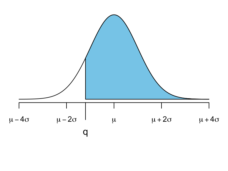
Visualize Probabilities

\(\Pr(X < 180)\) where \(X \sim N(170, 8)\)

pnorm(180, mean = 170, sd = 8)

[1] 0.8943502

\(\Pr(Z < 1.25)\) where \(Z \sim N(0, 1)\)

pnorm(1.25)

[1] 0.8943502

Finding Probabilities Using Z-scores

To find probabilites for \(X\sim N(\mu, \sigma)\)

1. Convert \(X\) to a \(Z\)-score:

   \[ Z = \frac{x - \mu}{\sigma} = z \]

2. Use the standard normal Z-table or R

   \(P(Z < z)\)	pnorm(z)
   \(P(Z > z)\)	pnorm(z, lower.tail = FALSE)
   \(P(a < Z < b)\)	pnorm(b) - pnorm(a)

Standardizing a Sample Mean

If we take a sample of size \(n\), the mean \(\bar{X}\) follows:

\[ \bar{X} \sim \text{Normal}\left(\mu_{\bar X} = \mu, \sigma_{\bar X} = \frac{\sigma}{\sqrt{n}}\right) \]

To standardize the sample mean:

\[ Z = \frac{\bar{X} - \mu_{\bar X}}{\sigma_{\bar X}} = \frac{\bar{X} - \mu_{\bar X}}{\sigma / \sqrt{n}} \]

This accounts for sampling variability. Used in hypothesis testing and confidence intervals.

Household Groceries (iClicker)

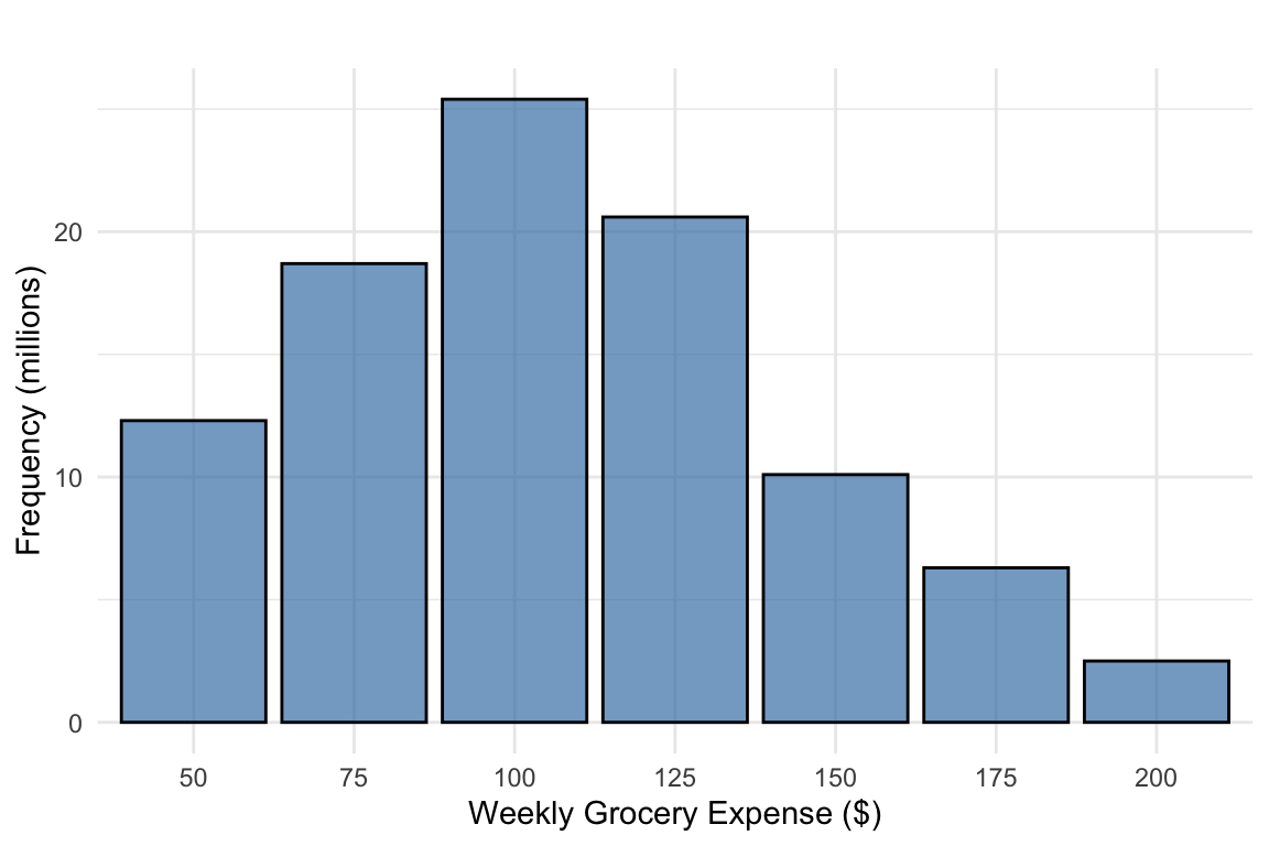
Exercise 1 Weekly Grocery Expenses The weekly grocery expenses for households in a certain region follow the the distribution given in Figure 1. According to a national consumer survey, the average grocery expense for this region is 107 with a standard deviation of \(38\). A random sample of 25 households is selected from this population.

What is the sampling distribution¹ of \(\bar X\)?

1. \(\bar X \sim N(0,1)\)
2. \(\bar X \sim N(107,38)\)
3. \(\bar X \sim N(107,38/25)\)
4. \(\bar X \sim N(107,38/\sqrt{25})\)
5. None of the above

Figure 1: Distribution of weekly grocery expesnse for housholds in a certain region.

1. We are using the \(N(\mu, \sigma)\) parameterization

✏️ Household Groceries

Exercise 2 Weekly Grocery Expenses The weekly grocery expenses for households in a certain region follow the the distribution given in Figure 1. According to a national consumer survey, the average grocery expense for this region is 107 with a standard deviation of \(38\). A random sample of 25 households is selected from this population.

Distribution of weekly grocery expesnse for housholds in a certain region.

What is the probability that the average weekly grocery expense for a randomly selected sample of 25 households exceeds $120?

Solution

We want \(\Pr(\bar X > 120)\) where the sample mean \(\bar{X}\) follows a normal distribution:

\[ \bar{X} \sim \text{Normal}(\mu_{\bar{X}} = 107, \sigma_{\bar{X}} = \frac{\sigma}{\sqrt{n}} = \frac{38}{\sqrt{25}} = 7.6) \]

We compute the standardized Z-score:

\[ Z = \frac{\bar X - \mu}{\sigma_{\bar{X}}} = \frac{120 - 107}{7.6} = 1.711 \]

Thus, the probability that the sample mean exceeds $120 is:

\[ P(\bar{X} > 120) = P(Z > 1.711) \]

Using the \(Z\)-table:

\[ P(Z > 1.711) = 1 - P(Z < 1.711) = 1 - 0.9564 \]

Final probability:

\[ P(\bar{X} > 120) = 0.0436 \]

Summary

🔹 Although the population distribution is skewed, the CLT tells us that the sampling distribution of \(\bar{X}\) can be approximated by a normal distribution when the sample size is sufficiently large.

🔹 We stanrdarize \(\bar X\) to find probabilities on the standard normal curve.

Note that this distribution is right-skewed.

Using simulation, check whether this holds for a sample size of 40.

1. Compute the mean and standard deviation of the sample mean.

2. Describe the shape of the sampling distribution.

3. If we simulated 1000 samples of 40 households and plotted the sample means, what would you expect the histogram to look like?

Sampling Distribution for Proportions

CLT for proportions

When observations are independent and the sample size is sufficiently large, the sample proportion \(\hat p\) is given by

\[ \hat p = \frac{X_1 + X_2 + \dots X_n}{n} \rightarrow N\left(\mu_{\hat p} = p, \sigma_{\hat p} = \sqrt{\frac{p(1-p)}{n}}\right) \]

Success-failure condition

In order for the Central Limit Theorem to hold, the sample size is typically considered sufficiently large when \(np \geq 10\) and \(n(1-p) \geq 10\) , which is called the success-failure condition.

i.e. the sample proportion is an unbiased estimator of the population proportion

\(\hat p\) is approximately normally distributed for large n.

The accuracy of the normal approximation depends on n and p.

If p is close to 0.5, the approximation is quite accurate, even for moderate n.

The farther p is from 0.5, the larger n must be for the approximation to be accurate.

As a rule of thumb, we want at least 10 successes and failures in our sample.

High School Graduation Rates in Canada (iClicker)

Exercise 3 According to the 2021 Canadian Census, 94% of Canadian adults have completed at least a high school education. Suppose a random sample of 800 Canadian adults is taken, and it is observed that 738 of them have completed high school. Which of the following is TRUE regarding population and sample proportions?

1. The 94% represents the sample proportion because it comes from the Census data.
   
2. The 94% is the population proportion, while the proportion calculated from the sample is the sample proportion.
   
3. The sample proportion can never be smaller than the population proportion if the sample is random.
   
4. Both 94% and the proportion calculated from the sample are considered population proportions.

High School Graduation Rates in Canada (iClicker)

Exercise 4 According to the 2021 Canadian Census, 94% of Canadian adults have completed at least a high school education. Suppose a random sample of 800 Canadian adults is taken, and it is observed that 738 of them have completed high school. Can the sampling distribution of \(\hat{p}\) be modeled as approximately normal?

1. No since the population proportion is too high for normal approximation to be valid.

2. No since we are not sampling from a normal population.

3. Yes since \(n > 30\)

4. Yes since both \(n*p\) and \(n*(1-p)\) > 10

High School Graduation Rates in Canada (iClicker)

Exercise 5 According to the 2021 Canadian Census, 94% of Canadian adults have completed at least a high school education. Suppose a random sample of 800 Canadian adults is taken, and it is observed that 738 of them have completed high school. What is the standard error of the sample proportion?

1. \(\dfrac{0.94(1-0.94)}{\sqrt{800}}\)

2. \(\sqrt{\dfrac{0.94(1-0.94)}{800}}\)

3. \(\sqrt{\dfrac{0.94(1-0.94)}{800}}\)

4. \(\sqrt{\dfrac{\frac{738}{800}(1-\frac{738}{800})}{800}}\)

High School Graduation Rates in Canada

Exercise 6 According to the 2021 Canadian Census, 94% of Canadian adults have completed at least a high school education. The 2016 Canadian Census reported that 81.7% of Canadian adults have a secondary or equivalent degree. What is the probability that the sample proportion from the 2021 population will be as small or smaller than 81.7%?

Solution

Sampling Distribution of Variance

Sampling Distribution of Variance

Let \(X_1, X_2, \dots, X_n\) be a random sample from a normal population with mean \(\mu\) and variance \(\sigma^2\). It can be shown that

\[\begin{align*} \dfrac{(n−1)S^2}{\sigma^2} \sim \chi^2_{(n-1)} \end{align*}\]

where \(\chi^2_{(n-1)}\) denotes a chi-squared distribution with \(n−1\) degrees of freedom.

Probability for the Sampling Distribution of \(S^2\)

Exercise 7 A study reports that the variance in weekly grocery expenses for Canadian households is \(\sigma^2=225\) dollars squared. Suppose a random sample of 15 households is taken, and their sample variance \(S^2\) is computed. What is the probability that the sample variance is greater than 275?

1. \(P(S^2 > 275) = P\left(\chi^2 > \frac{n \times 275}{\sigma^2}\right)\)

2. \(P(S^2 > 275) = P\left(\chi^2 < \frac{n \times 275}{\sigma^2}\right)\)

3. \(P(S^2 > 275) = P\left(\chi^2 > \frac{(n-1) \times 275}{\sigma^2}\right)\)

4. \(P(S^2 > 275) = P\left(\chi^2 < \frac{(n-1) \times 275}{\sigma^2}\right)\)

Probabilities for Chi-squared RV

Compute the Chi-Square Test Statistic¹

\[\chi^2=\frac{(n-1)s^2}{\sigma^2}=\frac{(15-1)\times 275}{275}=\frac{14\times 275}{275}\]

To find the probability we need the Chi-squared table or R

\[P(S^2 > 275) = P(\chi^2 > 17.111)\]

1. A test statistic is a numerical value calculated from a sample of data that is used in hypothesis testing.

\[ \begin{align} \phantom{x}\\ \phantom{x}\\ \phantom{x}\\ \end{align} \]

Note

The Chi-squared table gives upper tail probabilities.

\[ \begin{align} P(S^2 > 275) = &P(\chi^2 > 17.111)\\ \Pr(\chi^2 > 21.064) < &P(\chi^2 > 17.111) < \Pr(\chi^2 > 7.790) \\ .10 < &P(\chi^2 > 17.111) < .90 \\ \end{align} \]

Chisquared Visualized

Chisquared Visualized

Chisquared Visualized

Hence the \(\Pr(\chi^2_{14} > 17.1)\) should be bigger than 10% but smaller than 90%.

this might seem like a very big range but we’ll see later that this probability range will be good enough for our needs.

Chisquared probabilities in R

pchisq(q, df, lower.tail = TRUE)

q

vector of quantiles

df

degrees of freedom

lower.tail

logical; if TRUE (default), probabilities are \(\Pr(X \leq q)\) otherwise \(\Pr(X > q)\)

Solution

To find the probability:

\[P(S^2 > 275) = P(\chi^2 > 17.111)\]

Using R:

pchisq(17.111, df=14, lower.tail=FALSE)

[1] 0.2503109

\[P(S^2 > 275) = 0.2503\]

Thus, the probability that the sample variance \(S^2\) exceeds 275 is 0.2503.