Lecture 4: Sampling Distributions
STAT 205: Introduction to Mathematical Statistics
University of British Columbia Okanagan
Outline
\(\newcommand{\Var}[1]{\text{Var}({#1})}\)
In this lecture we will be covering
Introduction
- Based on the probabilistic foundations covered in STAT 203, this lecture will cover a fundamental concept in statistics that describes the behavior of the sampling distribution.
- Statistical inference aims to draw meaningful and reliable conclusions about a population based on a sample of data drawn from that population.
Example: loan* data
Let’s return to our
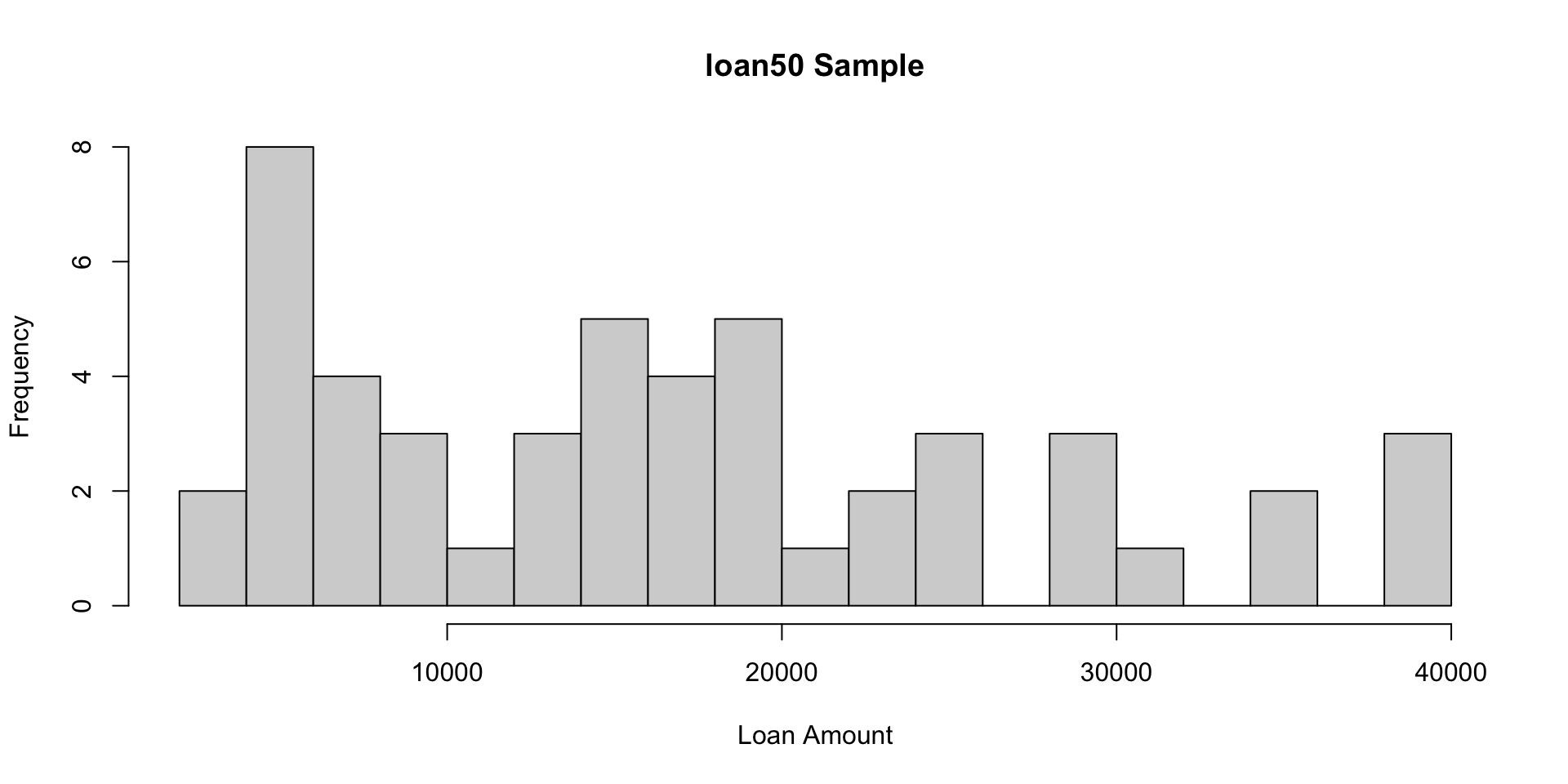
loan50example from previous lectures.This data set represents 50 loans made through the Lending Club platform, which is a platform that allows individuals to lend to other individuals.
Population data
The
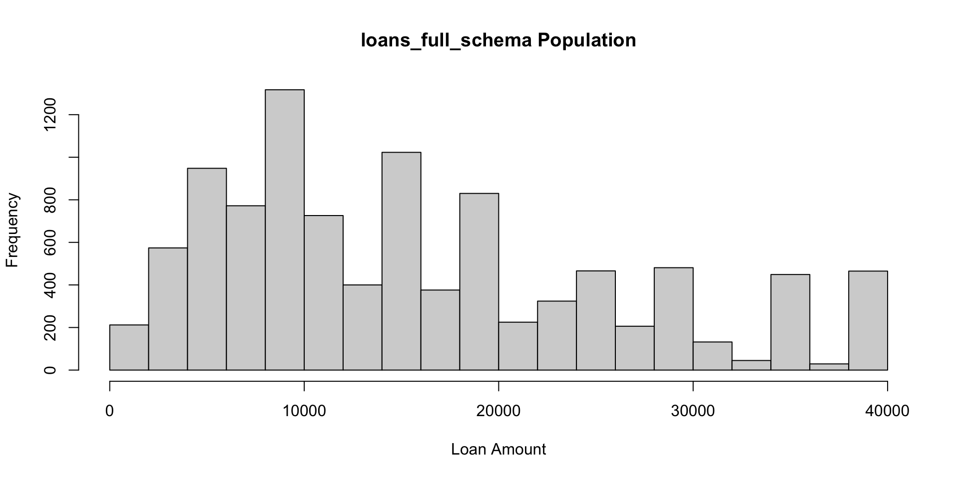
loans_full_schemacomprise 10,000 loans made through the Lending Club platform.Let’s pretend for demonstration purposes that this data set makes up all the loans made through the Lending Club and thus represents the population.
loan50is therefore a sample from that population.
Histogram: Population vs Sample
For the population we might be interested in some parameter, for example, the average loan amount, i.e. the mean value \(\mu\), and it’s standard deviation \(\sigma\).
Parameters
While the population mean is not usually possible to compute, since we have the data for the entire population we can easily calculate it using:
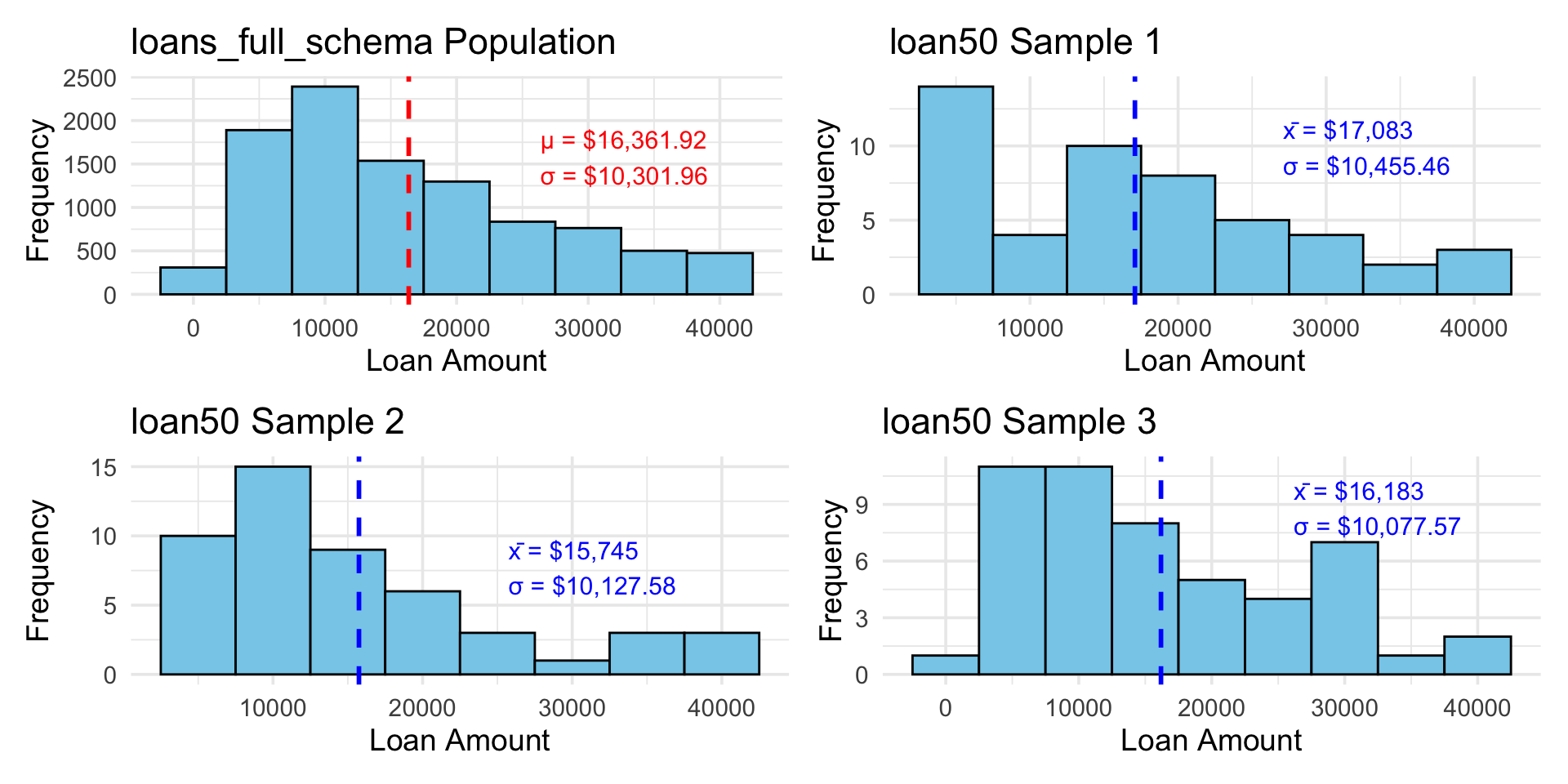
There average loan amount is $16,361.92
The standard deviation is $10,301.96
If we did not have access to the population information (as is often the case) and instead only had access to a sample, we would instead compute the sample mean:
There sample average loan amount is $17,083.00
The sample standard deviation is $10,455.46
Random Samples in R
Of course, a different random sample of 50 loans will produce a different sample mean:
N = nrow(loans_full_schema) # 10,000 observations
sampled50_loans <- loans_full_schema[sample(N, 50), ]
(mean_loan_amount <- mean(sampled50_loans$loan_amount))
[1] 15745There sample average loan amount is $15,745.00
Sampling Distribution of the mean
Let’s repeat this process many times and keep track of all of the sample mean calculations (one for each sample).
mean_vec = NULL
for (i in 1:1000) {
  sampled50_loans <- loans_full_schema[sample(N, 50), ]
  mean_vec[i] <- mean(sampled50_loans$loan_amount)
}
mean_vec[1:20]
[1] 16227.0 16194.0 16127.5 16297.5 13865.0 16121.0 18582.0 15622.5 16526.5
[10] 16262.0 18015.0 17969.5 17211.0 15508.5 19218.0 17669.5 16795.0 16488.0
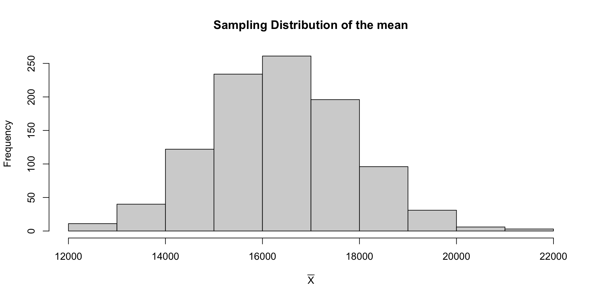
[19] 18747.5 16850.5...The distribution of the sample means is an example of a sampling distribution.
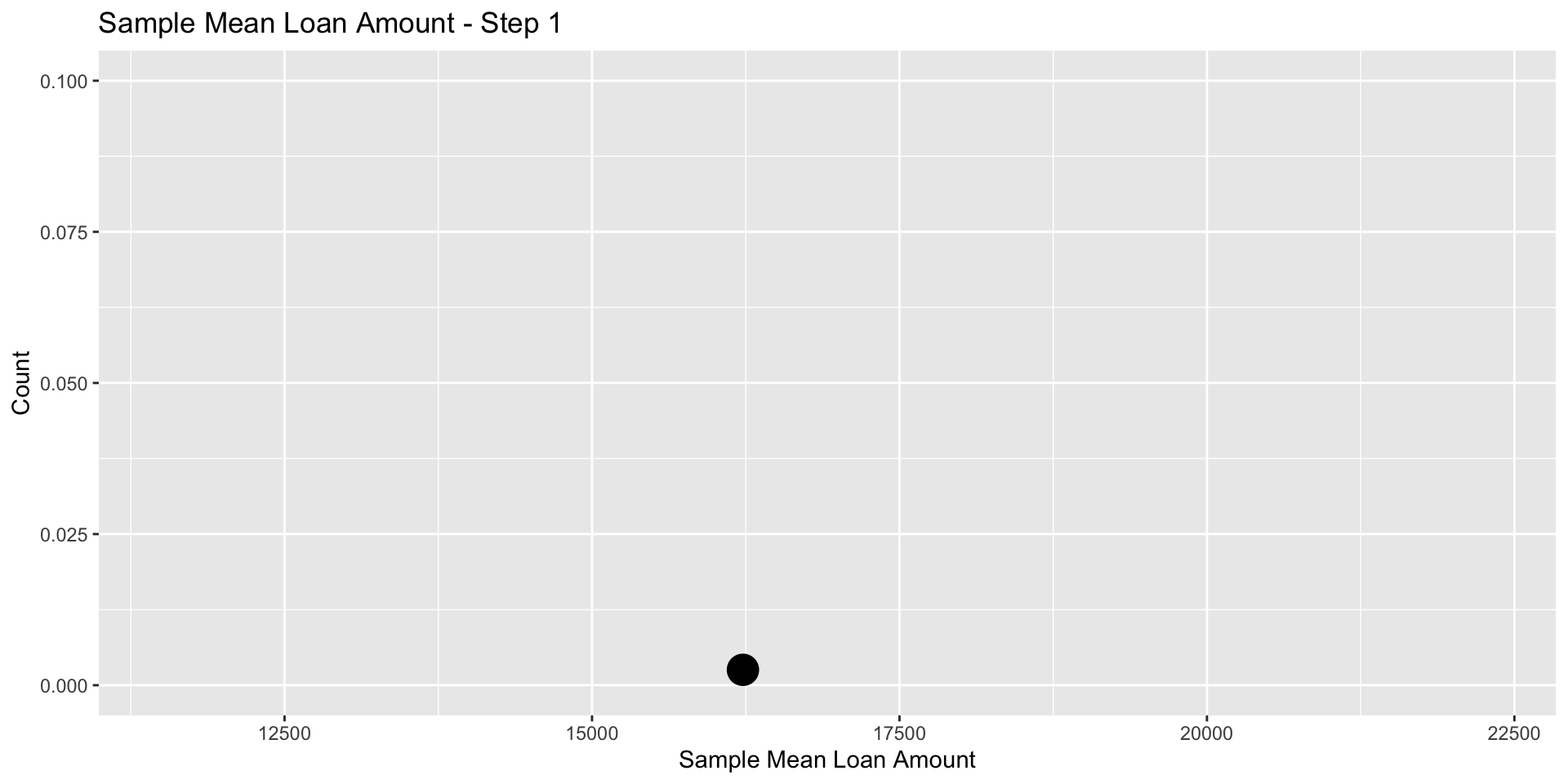
For the first sample, \(\bar x_1\) = 16227
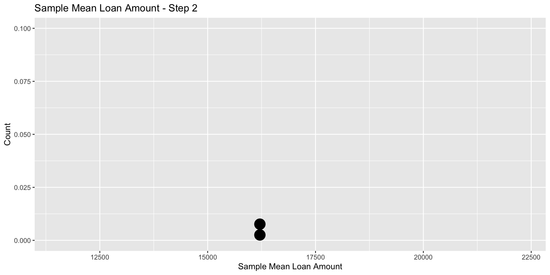
For the second sample, \(\bar x_2\) = 16194
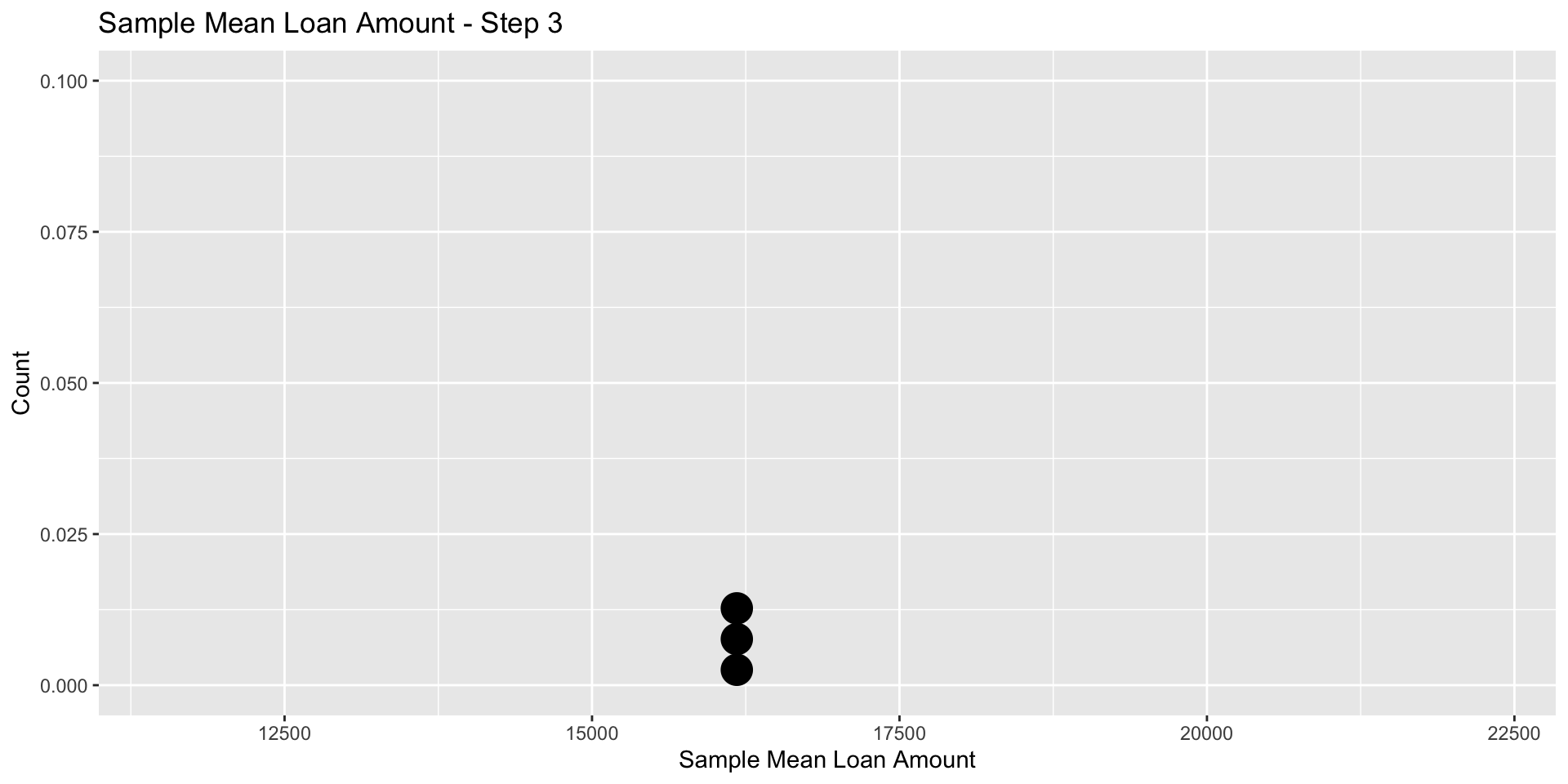
For the third sample, \(\bar x_3\) = 16127.5
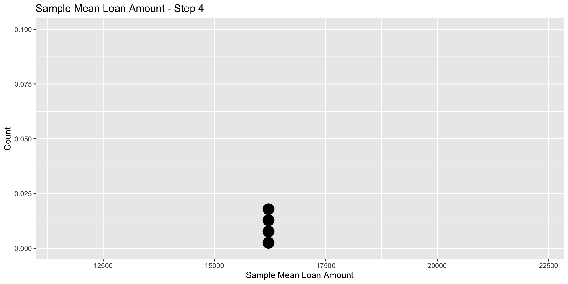
For the forth sample, \(\bar x_4\) = 16297.5
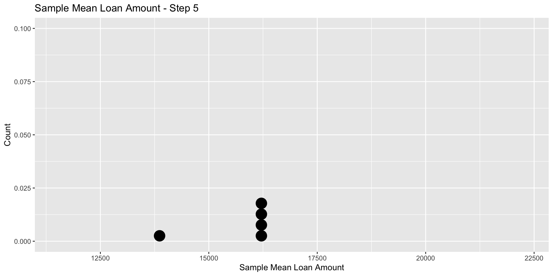
For the fifth sample, \(\bar x_5\) = 13865

For the sixth sample, \(\bar x_6\) = 16121
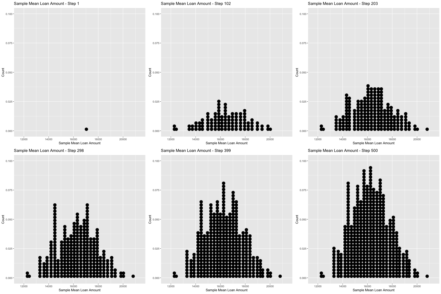
Empirical Sampling Distribution
To get so-called empirical estimate of that distribution we can plot a histogram of it’s values
Theoretical Sampling Distribution
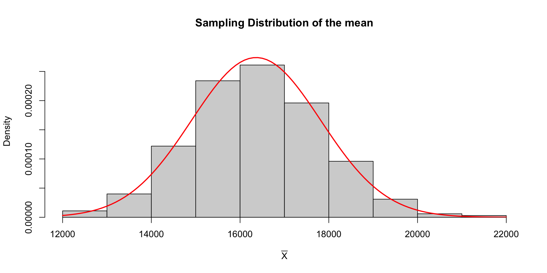
Thanks to the Central Limit Theorem we actually know what the theoretical probability distribution of \(\overline{X}\) is …
Theoretical Sampling Distribution
Thanks to the Central Limit Theorem we actually know what the theoretical probability distribution of \(\overline{X}\) is …
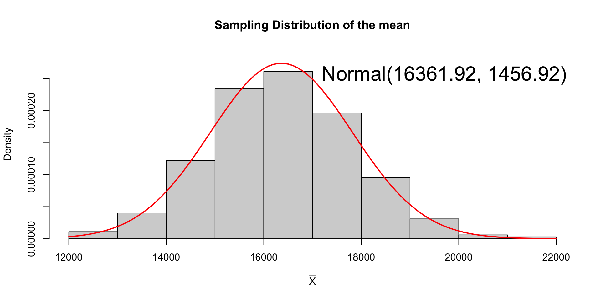
CLT for the Sample Mean
This phenomenon is known as the Central Limit theorem.
It says the probability distribution of \(\overline{X}\) approaches a Normal distribution as long as the sample size is large enough1.
The mean (expected value) of the sampling distribution of the sample mean is equal to the population mean (\(\mu\)) and the standard deviation (more commonly referred to as the standard error) is \(\sigma_\overline{X} = \frac{\sigma}{n}\). We often write:
\[ \begin{equation} \overline{X} \sim N(\mu_\overline{X} = \mu, \sigma_\overline{X} = \sigma/n) \end{equation} \]
iClicker
Understanding Sampling Distributions
A sampling distribution represents:
The distribution of a sample.
The distribution of a population.
The distribution of a statistic, like the sample mean, across repeated samples.
The distribution of a parameter, like the population mean.
iClicker
Central Limit Theorem
According to the Central Limit Theorem, the sampling distribution of the sample mean:
Always follows a normal distribution regardless of sample size.
Becomes approximately normal as the sample size increases.
Becomes approximately normal as the number of samples increase.
Has a standard deviation equal to the population standard deviation.
Is skewed when the population distribution is skewed.
iClicker
Variability of the Sample Mean
As the sample size increases, the variability of the sample mean:
Increases.
Decreases.
Remains constant.
Depends on the population distribution.
Random Sample
Definition: Sample
If \(X_1, X_2, \dots, X_n\) are independent random variables (RVs) having a common distribution \(F\), then we say that they constitute a sample (sometimes called a random sample) from the distribution \(F\).
- Oftentimes, \(F\) is not known and we attempt to make inferences about it based on a sample.
- Parametric inference problems assume \(F\) follows a named distribution (e.g. normal, Poisson, etc) with unknown parameters.
Statistic
Definition: (Sample) Statistic
Let’s denote the sample data as \(X = (X_1, X_2, \dots, X_n)\) , where \(n\) is the sample size. A statistic, denoted \(T(X)\), is a function of a sample of observations.
\[ T(X) = g(X_1, X_2, \dots, X_n) \]
- A prime example of a statistic is the sample mean and sample variance
- Understanding that these are both RV, we can calculate things like their Expected value.
Sampling Distribution
Definition: Sampling Distribution
A sampling distribution is the probability distribution of a given a sample statistic.
In other words, if were were to repeatedly draw samples from the population and compute the value of the statistic (e.g. sample mean, or variance), the sampling distribution is the probability distribution of the values that the statistic takes on.
Important
In many contexts, only one sample is observed, but the sampling distribution can be found theoretically.
Review of CLT
Central Limit Theorem
Let \(X_1, X_2, \dots, X_n\) be a sequence of independent and identically distributed (i.i.d) RVs each having mean \(\mu\) and variance \(\sigma^2\). Then for \(n\) large, the distribution of the sum of those random variables is approximately normal with mean \(n\mu\) and variance \(n\sigma^2\)
\[ \begin{align*} X_1 + X_2 + \dots + X_n &\sim N(n\mu, n\sigma^2) \end{align*} \]
\[ \begin{align*} \dfrac{X_1 + X_2 + \dots + X_n}{n} &\sim N\left(\mu, \dfrac{\sigma^2}{n}\right) \end{align*} \]
\[ % Z_n = \dfrac{X_1 + \dots + X_n - n\mu}{\sigma/\sqrt{n}} = \dfrac{\sum_{i=1}^n X_i - \mu}{\sigma/\sqrt{n}} \rightarrow N(0,1) Z_n = \dfrac{\overline{X} - \mu}{\sigma/\sqrt{n}} \rightarrow N(0,1) \text{ as } n \rightarrow \infty \]
However, the rate of shrinking is exactly balanced in such a way that their ratio remains a random variable with constant variance.
Sample Mean
A prime example of a sample statistic is the sample mean:
\[ \overline{X} = \dfrac{X_1 + X_2 + \dots, + X_n}{n} \]
This is simply another RV having it’s own:
- expected value \(\mathbb{E}[\overline{X}]\) (i.e. “mean of the sampling mean”)
- variance \(\Var{\overline{X}}\)
- and distribution (i.e. sampling distribution)
Expected Value of the Sample Mean
Assuming \(X_i \overset{\mathrm{iid}}{\sim} F\) where \(F\) has a mean of \(\mu\) and variance \(\sigma^2\):
\[ \begin{align*} \class{fragment}{\mathbb{E}[\overline{X}]} &\class{fragment}{{} = \mathbb{E}\left[\dfrac{X_1+ \dots X_n}{n}\right]} \\ &\class{fragment}{{} = \dfrac{\mathbb{E}[X_1]+ \dots \mathbb{E}[X_n]}{n}} \\ &\class{fragment}{{} = \dfrac{\sum_{i=1}^n \mathbb{E}[X_i]}{n}} \\ &\class{fragment}{{} = \dfrac{n\mu}{n}} \class{fragment}{{} = \mu} \end{align*} \]
Variance of the Sample Mean
\[ \begin{align*} \text{Var}\left(\overline{X}\right) &\class{fragment}{{} = \text{Var}\left(\frac{X_1 + \dots + X_n}{n}\right)} \\ & \class{fragment}{{} \text{by independence ...}}\\ & \class{fragment}{{} = \frac{1}{n^2} \left[\text{Var}(X_1) + \dots + \text{Var}(X_n)\right]} \\ & \class{fragment}{{} = \frac{n \sigma^2}{n^2} = \frac{\sigma^2}{n}} \end{align*} \]
Rolling a die
Example: Rolling a die
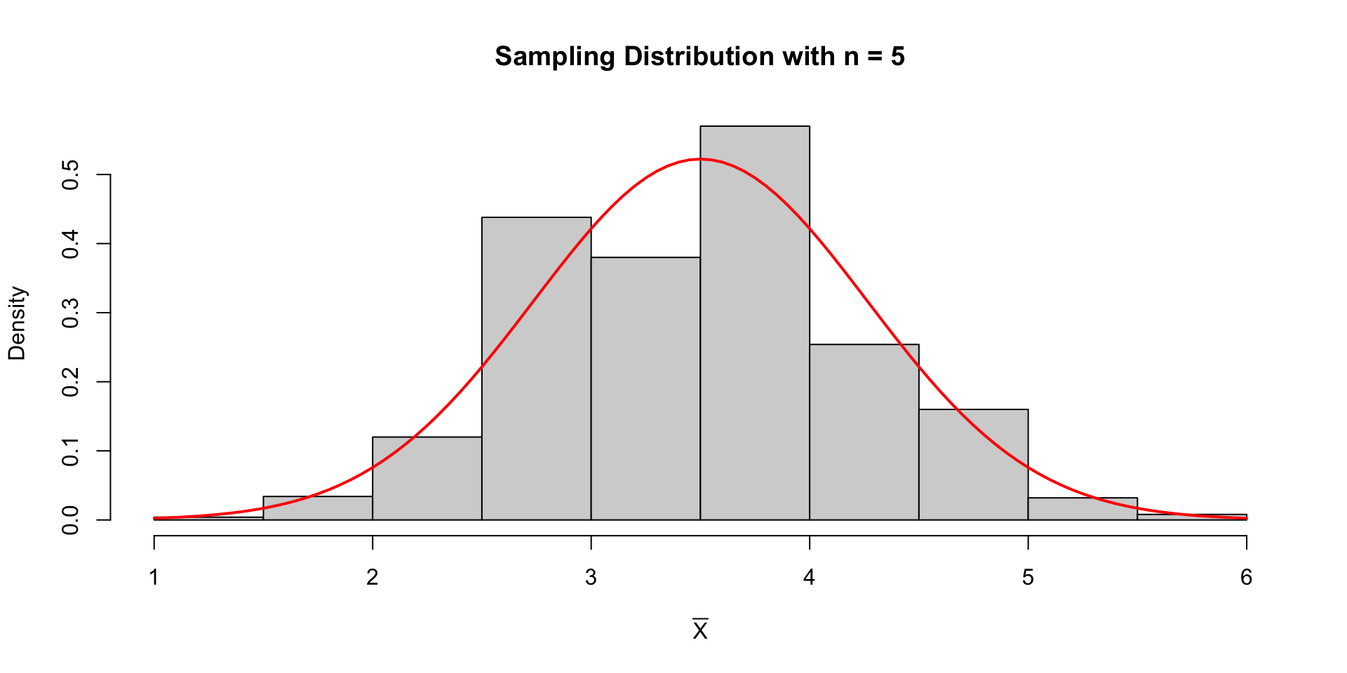
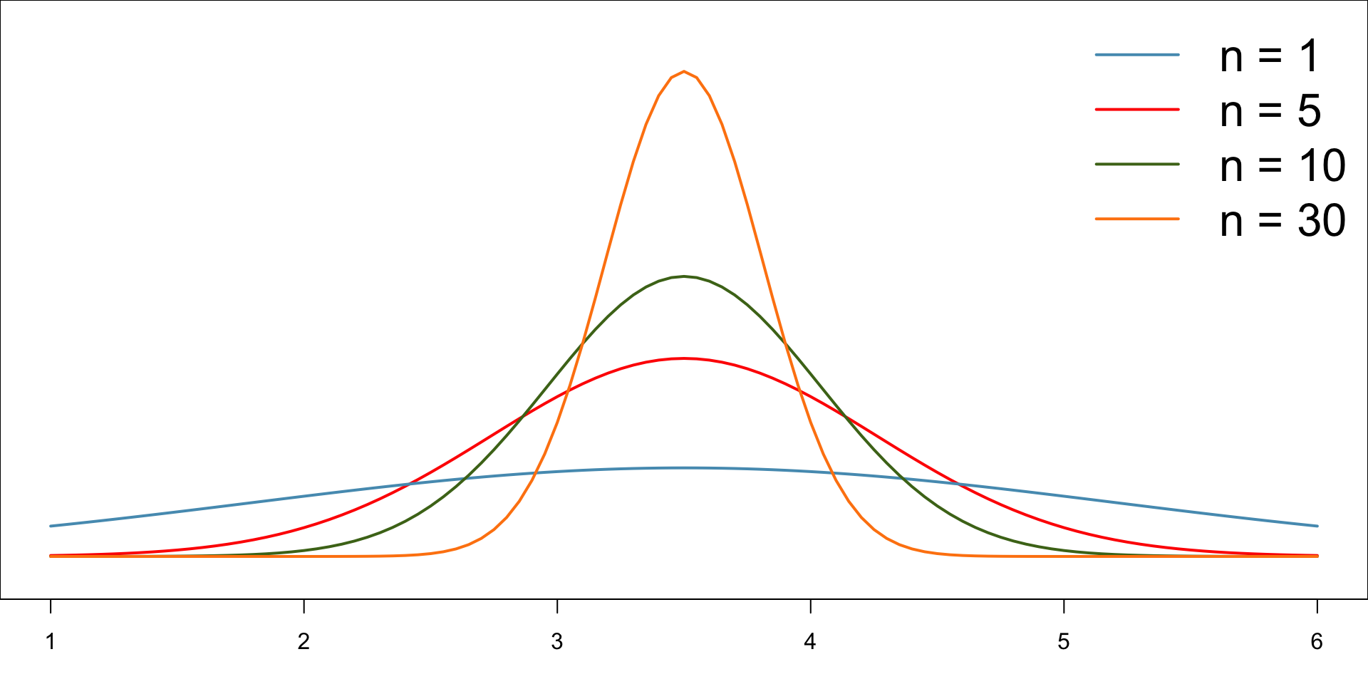
What is the sampling distribution of the mean of 5 rolls of a dice? \(\overline{X} \sim ?\)
We first need to identify the distribution of \(X_i\)
Mean and standard error
Theoretical Result
Let \(X_i\) be the number of dots facing up when rolling a fair die.
Let \(\overline{X} = \frac{X_1 + X_2 + \dots X_5}{5}\) be the mean of five rolls.
Then from the CLT we know: \[ \begin{align*} \overline{X} &\sim N(\mu_{\overline{X}} = 3.5, \sigma_{\overline{X}} = \frac{\sqrt{((6-1+1)^2 -1)/12)}}{\sqrt{5}})\\ &\sim N(\mu_{\overline{X}} = 3.5, \sigma_{\overline{X}} = 0.7637626) \end{align*} \]
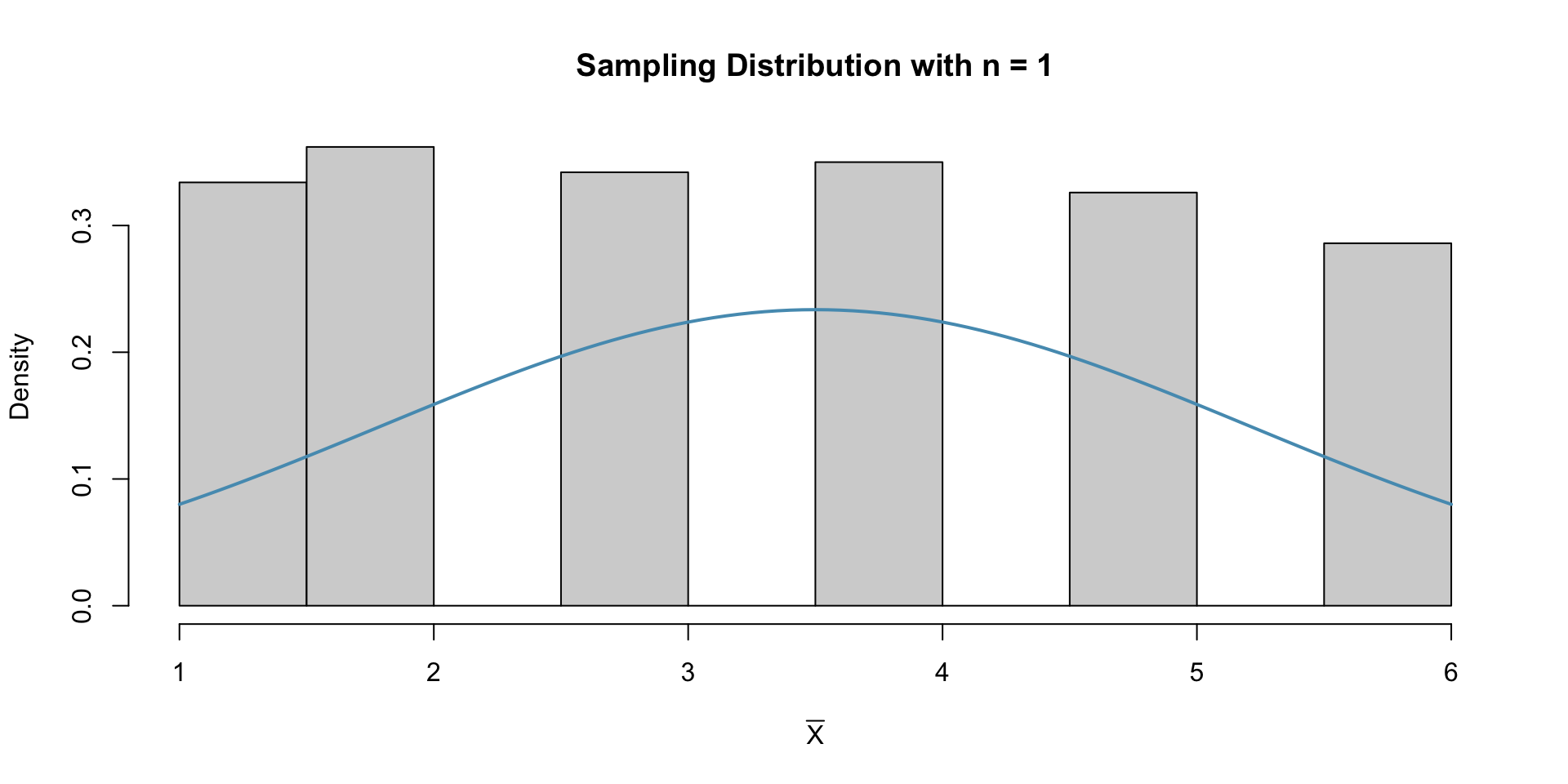
Empirical Result
n = 1
n = 10

n = 30
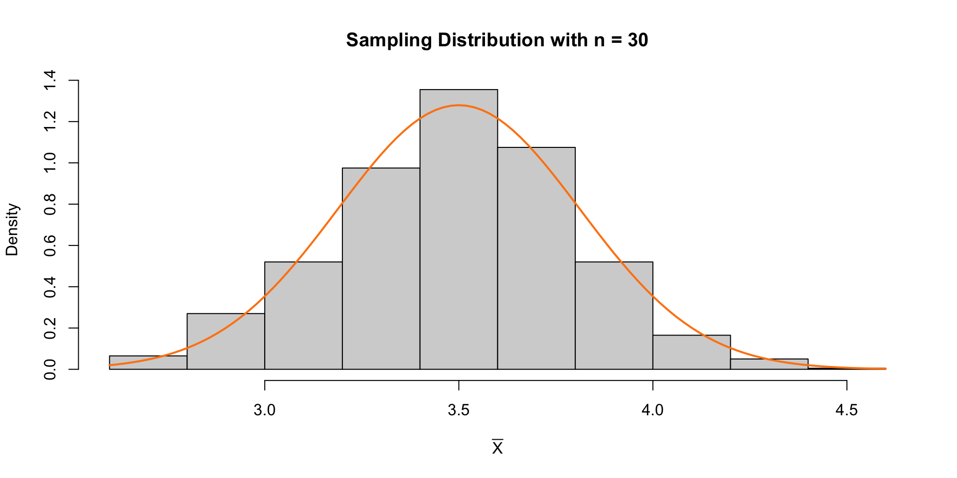
Difference Sample Sizes
Solar Energy Example
Example: Solar Energy
Suppose we are interested in the proportion of American adults who support the expansion of solar energy. Suppose we don’t have access to the population of all American adults, which is a quite likely scenario, and we sample 1000 American adults and 895 approve of solar energy. What is the sampling distribution of the proportion?
Sampling Distribution for Proportions
CLT for proportions
When observations are independent and the sample size is sufficiently large, the sample proportion \(\hat p\) is given by
\[ \hat p = \frac{X_1 + X_2 + \dots X_n}{n} \rightarrow N\left(\mu_{\hat p} = p, \sigma_{\hat p} = \sqrt{\frac{p(1-p)}{n}}\right) \]
Success-failure condition
In order for the Central Limit Theorem to hold, the sample size is typically considered sufficiently large when \(np \geq 10\) and \(n(1-p) \geq 10\) , which is called the success-failure condition.
Standard error of proportion
\[\begin{align*} \sigma_{\hat p} &= \sqrt{\frac{p(1-p)}{n}} \end{align*}\]
To approximate this we sub \(p\) (the unknown population parameter) with the point estimate \(\hat p\): \[\begin{align*} \hat{\sigma_{\hat p}} &\approx \sqrt{\frac{\hat p(1-\hat p)}{n}} \\ \end{align*}\]
This is sometimes called the plug-in principal.
Empirical Sampling distribution of Proportion
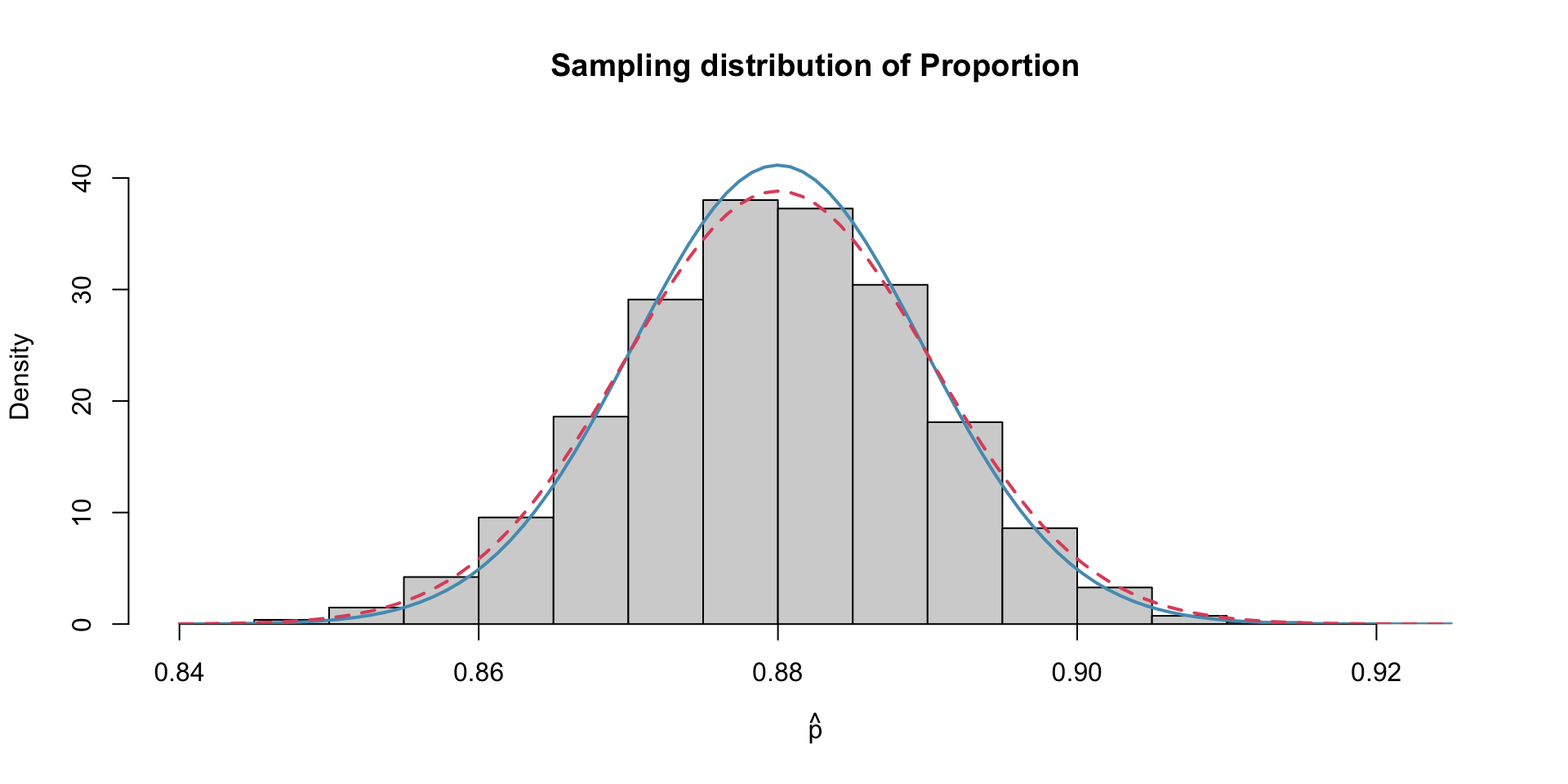
Because I have simulated this data, we can compare the empirical sample distribution to the theoretical sampling distribution (red) with the sampling distribution using the estimate of standard error (blue)
Sampling Distribution of Variance
The sample variance, \(S^2\), is yet another sample statistic which we define as \[S^2 = \frac{\sum_{i=1}^{n} (X_i - \overline{X})^2}{n-1}\]
It can be shown that this is an unbiased estimate for \(\sigma^2\), i.e. \[\mathbb{E}[S^2] = \sigma^2\]
Expected value of Variance
Using the following algebric result (see Proof):
\[ \sum_{i=1}^{n} \left( x_i - \overline{x} \right)^2 = \sum_{i=1}^{n} x_i^2 - n\overline{x}^2 \] we can rewrite the statistic as:
\[ (n-1) S^2 = \sum_{i=1}^{n} (X_i - \overline{X})^2 = \sum_{i=1}^{n}X_i^2 - n \overline{X}^2 \]
Proof
\[\begin{align*} \sum_{i=1}^{n} \left( x_i - \overline{x} \right)^2 &= \sum_{i=1}^{n} \left( x_i^2 - 2x_i\overline{x} + \overline{x}^2 \right) \\ &= \sum_{i=1}^{n} x_i^2 - 2\overline{x} \sum_{i=1}^{n} x_i + \sum_{i=1}^{n} \overline{x}^2 \\ &= \sum_{i=1}^{n} x_i^2 - 2\overline{x} (n\cdot \overline{x}) + n\cdot \overline{x}^2 \\ &= \sum_{i=1}^{n} x_i^2 + \overline{x}^2(n - 2n) \\ &= \sum_{i=1}^{n} x_i^2 - n\overline{x}^2 \end{align*}\]
Expected value of Variance (cont’d)
Taking the expectation of both sides … \[ (n-1)\mathbb{E}[S^2] = \mathbb{E}\left[\sum_{i=1}^{n} X_i^2\right] - n\mathbb{E}[\overline{X}^2] \] Recall for any random variable \(W\), \(\mathbb{E}[W^2] = \text{Var}(W) + (\mathbb{E}[W])^2\) \[\begin{align*} &= n\text{Var}(X_i) + \left(\sum_{i=1}^n \mathbb{E}[X_i]\right)^2 - n\left( \text{Var}(\overline{X}) + (\mathbb{E}[\overline{X}])^2 \right)\\ &= n\sigma^2 + n\mu^2 - n \text{Var}(\overline{X}) - n\mu^2 \\ &= n\sigma^2 - n \text{Var}(\overline{X}) \\ &= n\sigma^2 - n \frac{\sigma^2}{n} = (n-1)\sigma^2 \end{align*}\]
Or \(E[S^2] = \frac{(n-1)\sigma^2}{(n-1)} = \sigma^2\)
Sampling Distribution of Variance
Normal Population
Let \(X_1, X_2, \dots, X_n\) be a random sample from a normal distribution with mean \(\mu\) and variance \(\sigma^2\). It can be shown that
\[\begin{align*} \dfrac{(n−1)S^2}{\sigma^2} \sim \chi^2_{(n-1)} \end{align*}\] where \(\chi^2_{(n-1)}\) denotes a chi-squared distribution with \(n−1\) degrees of freedom.
Normality Assumption
Warning
It’s important to note that this result holds under the assumption of normality for the underlying population. If the population is not normal, the distribution of the sample variance may still be approximately chi-squared if the sample size is sufficiently large due to the central limit theorem.
Simulation 1: Normal Population
Example: Chi-square simulation (Normal population)
Suppose we take 10000 samples of size \(n =\) 5 from a normal population with \(\sigma^2 =\) 1. Plot the empirical distribution from 10000 runs alongside the theoretical distribution of \(\frac{(n-1)S^2}{\sigma^2}\).
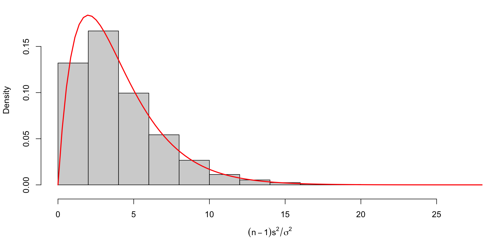
n = 10
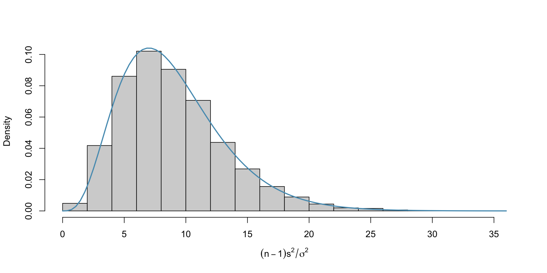
n = 20

n = 100
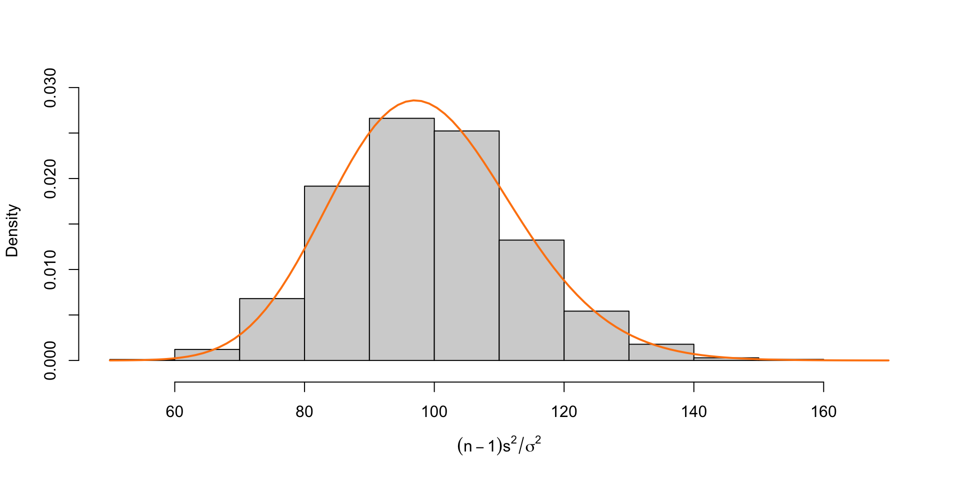
Simulation 2: Uniform Population
Example: Chi-square simulation (Uniform population)
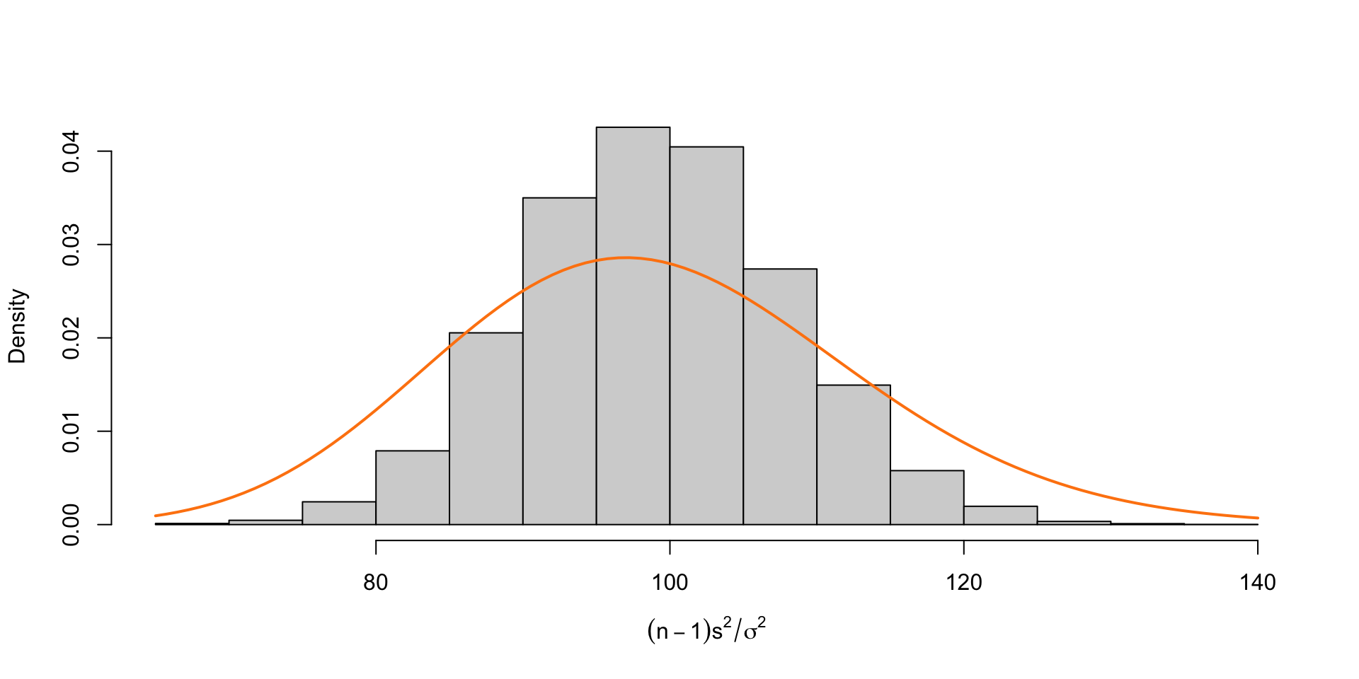
Suppose we take 10000 samples of size \(n =\) 5 from a uniform population with \(\sigma^2 =\) 1. Plot the empirical distribution of \(\frac{(n-1)S^2}{\sigma^2}\) from 10000 runs alongside the theoretical distribution of \(\frac{(n-1)S^2}{\sigma^2}\) if the population were normal.

n = 10
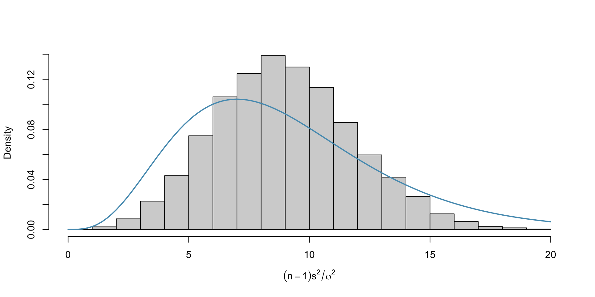
n = 20

n = 100
