Inference for Two Sample Means

STAT 205: Introduction to Mathematical Statistics

Dr. Irene Vrbik

University of British Columbia Okanagan

Introduction

So far we have covered statistical inference methods involving various population parameters from a single population. However, studies often compare two groups. For example:

• Comparative Analysis: investigating differences in outcomes, characteristics, or behaviors between different groups.

• Treatment Comparisons: In experimental or intervention studies, researchers often want to evaluate the effectiveness of different treatments or interventions.

• Before-and-After Studies: In longitudinal or repeated measures studies, researchers may measure the same group of individuals before and after an intervention or treatment.

1. Comparative Analysis: It allows researchers to assess whether there is a significant difference between the means of two populations or groups. This comparison is useful for investigating differences in outcomes, characteristics, or behaviors between different groups.

2. Treatment Comparisons: In experimental or intervention studies, researchers often want to evaluate the effectiveness of different treatments or interventions. Comparing the means of outcome variables between treatment groups helps determine which treatment is more effective.

3. Before-and-After Studies: In longitudinal or repeated measures studies, researchers may measure the same group of individuals before and after an intervention or treatment. Inference on the difference between means allows researchers to assess whether there has been a significant change over time.

4. Controlled Experiments: In controlled experiments, researchers may manipulate an independent variable (e.g., treatment, condition) and measure its effect on a dependent variable. Inference on the difference between means helps determine whether the observed differences are statistically significant and not due to random variation.

5. Matched Case-Control Studies: In matched case-control studies, researchers match cases (individuals with a particular condition or outcome) with controls (individuals without the condition) based on certain characteristics. Inference on the difference between means helps assess whether there are significant differences in characteristics between cases and controls.

Motivation

We will now introduce inference procedures for the difference of two population means which may wish to investigate questions like:

• Are there differences in average test scores between students who received traditional instruction and those who participated in a new teaching method?

• Is there a significant difference in blood pressure levels between patients who received a new medication and those who received a placebo?

• Do employees who undergo a new training program exhibit higher productivity levels compared to employees who did not undergo the training?

Advancements in various fields, including science and engineering, often stem from the invention of new devices, materials, or the revision of existing processes. These advancements occur when a new technique demonstrates superiority over the old methods.

To evaluate the effectiveness of these innovations, experiments are conducted, and data on their performance is collected. Statistical methods are then employed to compare the performance of the new techniques with the old ones, aiding in the assessment of their relative merits.

Parallels with One-Sample Inference

When doing inference on mean of one population (having unknown mean \(\mu\) and variance \(\sigma^2\)), we leveraged the theoretical knowledge of the sampling distribution of it’s estimator, i.e. the mean of a sample of size \(n\):

\[ \bar{X} \sim \text{Normal}(\mu_{\bar{X}} = \mu, SE = \sigma/\sqrt{n}) \]

We can then standardize this random variable and calculate probabilities and quantiles using the standard normal distribution which we use to make inferential decisions.

We know the mean of sample of \(n\) observations taken from a population with mean \(\mu\) and standard deviation \(\sigma\) follows as normal distribution. Namely:

Population Parameter of Interest

• Now, we consider the very common problem of comparing two population means.

• These formal hypothesis tests provide a structured framework to investigate whether or not the two groups differ from each other. Hence, we are interested in

  \[ \mu_1 - \mu_2 \]

  where \(\mu_1\) and \(\mu_2\) is the population mean from group 1 and 2, respectively.

Is the night shift less productive than the day shift, are the rates of return from fixed asset investments different from those from common stock investments, and so on?

Concepts

• As before, the population parameters are not obtainable and we therefore need to estimate them from a sample – in this case, samples – from the populations of interest.

• Unsurprisingly, \(\bar{X}_1 - \bar{X}_2\) will be the estimator of \(\mu_1 - \mu_2\).

• To do inference, we will need to determine the sampling distribution of \(\bar{X}_1 - \bar{X}_2\) which we can transform into a test statistic (or pivot) that we may use in our formal tests.

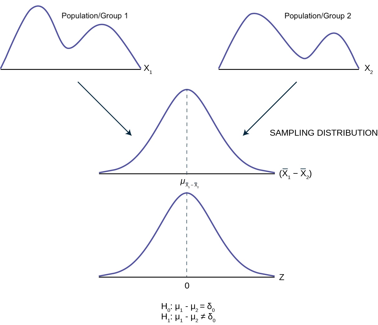
Image adapted from OpenStax Figure 10.2

Top: two distributions of data, X₁ and X₂, with unknown means and standard deviations.

Middle: the sampling distribution of the newly created random variable (\(X_1 - X_2\)); this is the theoretical distribution of many sample means from population 1 minus sample means from population 2.

CTL tells us this sampling distribution is normally distributed, regardless of the distribution of the actual population data shown in the top panel.

We can now standardize and calculate probabilities from the standard normal as before.

Considerations

• As it turns out, the observed difference between two sample means depends on both the means and the sample standard deviations.

• Very different means can occur by chance if there is great variation among the individual samples and the test statistic will have to account for this fact.

• Furthermore, we have different tests for when the groups are independent vs matched /paired.

Notation

• We denote \(\bar{X}_1\) as the mean of a random sample of size \(n_1\) from population 1 having mean \(\mu_1\) and variance \(\sigma_1^2\).

• Similarly let \(\bar{X}_2\) be the mean of a random sample of size \(n_2\) from a second population having mean \(\mu_2\) and variance \(\sigma_2^2\).

The first thing we need to ask ourselves is: are the two populations are independent?

Independent Populations

In this context, two populations are considered independent when the observations or measurements in one population are not related to or dependent on the observations or measurements in the other population.

• e.g. patients in a treatment group receiving a new drug are independent of those in the control group receiving a placebo.

• e.g. heights of individuals in one country are independent of heights of individuals in the other country.

• In other words, the individuals or items sampled from one population are unrelated to those sampled from the other population.

• Analyzing the heights of adults in two different countries:: The height of one person does not depend on the height of someone from another country.

Dependent Populations

• Dependent populations is where the observations in one group are paired or matched with corresponding observations in the other group.

• These pairs are linked in some way, and the relationship between them is of interest in the analysis.

• A common case is repeated measurement designs in which participants are measured multiple times under different conditions/time points.

  • e.g. tracking the performance of athletes before and after a training regimen.

Sampling from Dependent Groups

The dependent groups \(t\)-test is exactly the same as the one-sample \(t\)-test procedure for a single population …

\(X_1\)	\(X_2\)	\(d\)
\(x_{11}\)	\(x_{21}\)	\(d_1 = x_{11} - x_{21}\)
\(x_{12}\)	\(x_{22}\)	\(d_2 = x_{12} - x_{22}\)
\(\vdots\)	\(\vdots\)	\(\vdots\)
\(x_{1n}\)	\(x_{1n}\)	\(d_n = x_{1n} - x_{2n}\)

… only now, our sample consists of \(d_1, d_2, \dots, d_n\)

Sampling from Independent Groups

Sampling Distribution of the Difference in Sample Means

If we are sampling from independent populations, then

\[\begin{equation} \bar X_1 - \bar X_2 \sim \text{Normal} \left(\mu_1 - \mu_2, SE = \sqrt{ \frac{\sigma_1^2}{n_1} + \frac{\sigma_2^2}{n_2} } \right) \end{equation}\] This will be exact when we are sampling from a normal population (even for small sample sizes). This will be approximate for large ( \(n\) \(\geq 30\)) samples from non-normal populations thanks to CLT.

Independent Groups Assumptions

Assumptions with Large Samples

1. \(X_1 = (X_{11}, X_{12}, \dots, X_{1n_1})\) is a random sample of size \(n_1\) from population/group 1 having a mean and variance of \(\mu_1\) and \(\sigma^2_1\), respectively.
2. \(X_2 = (X_{21}, X_{22}, \dots, X_{2n_2})\) is a random sample of size \(n_2\) from population/group 1 having a mean and variance of \(\mu_2\) and \(\sigma^2_2\), respectively.
3. The two samples \(X_1\) and \(X_2\) are independent.

Inferences will be made on \(\mu_1 - \mu_2 = \delta\)

For we consider two independent samples when both sample sizes are large.

Test Statistic (known variances)

Two-sample Z statistic

If we are sampling from independent populations, and doing inference on \(\mu_1 - \mu_2 = \delta\) then the two sample \(Z\)-statistic is given by:

\[ Z = \dfrac {\bar{X}_1 - \bar{X}_2 - \delta} {\sqrt{ \dfrac{\sigma_1^2}{n_1} + \dfrac{\sigma_2^2}{n_2} }} \] follows a standard normal distribution. This will be exact when we are sampling from a normal population (even for small sample sizes). This will be approximate for large ( \(n\) \(\geq 30\)) samples from non-normal populations thanks to CLT.

all this is is normalizing the sampling dist of \(\bar X_1 - \bar X_2\)

Test Statistic (unknown variances)

Two-sample t-statistic

If we are sampling from independent populations, and doing inference on \(\mu_1 - \mu_2 = \delta\) then the two sample \(Z\)-statistic is given by:

\[ T = \dfrac {\bar{X}_1 - \bar{X}_2 - \delta} {\sqrt{ \dfrac{S_1^2}{n_1} + \dfrac{S_2^2}{n_2} }} \] follows a student \(t\)-distribution¹. The degrees will depend on whether or not we assume the variance of the two groups are equal, i.e. \(\sigma_1 = \sigma_2\).

Recall that in one-sample inference procedures for μ, we replaced the population standard deviation in the Z statistic with the sample standard deviation (σ is replaced by s), and this resulted in a t statistic.

Although we will do something similar here, there is an added complication

1. this will be exact if we assume \(\sigma_1^2 = \sigma_2^2\), otherwise, approximate.

df (Equal Variance)

• When we assume \(\sigma_1 = \sigma_2\), we may follow the exact procedure called the pooled \(t\)-test (aka two-sample \(t\)-test).

• In this case the test statistic \(T\) is exactly \(t\)-distributed with degrees of freedom equal to

\[ \nu = n_1 + n_2 - 2 \]

df (Unequal Variance)

• When it is not safe to assume \(\sigma_1 = \sigma_2\), we follow an approximateprocedure called the Welch procedure.

• In this case the test statistic \(T\) is approximately \(t\)-distributed with degrees of freedom equal to

\[ \nu = \dfrac{\left( \frac{s_1^2}{n_1} + \frac{s_2^2}{n_2} \right)^2}{\frac{1}{n_1 - 1}\left( \frac{s_1^2}{n_1} \right)^2 + \frac{1}{n_2 - 1} \left( \frac{s_2^2}{n_2} \right)^2}\]

Sample variances (equal variance)

When we assume \(\sigma_1 = \sigma_2\), we may estimate \(\sigma_1^2\) and \(\sigma_2^2\) by the so-called pooled sample variance given by:

\[ s_p^2 = \dfrac{(n_1 - 1)s_1^2 + (n_2 - 1)s_2^2}{n_1 + n_2 -2} \]

This will estimate the common variance \(\sigma^2 = \sigma_1^2 = \sigma_2^2\).

This is simply a weighted average of the two sample variances.

it will be an exact average if the sample sizes are the same,

otherwise, it will be a little closer to one sample variance that has more observations

Sample variances (unequal variance)

When it is not safe to assume \(\sigma_1 = \sigma_2\), we will estimate \(\sigma^2_1\) and \(\sigma^2_2\) in the usual way, namely:

\[\begin{align} s_1^2 &= \dfrac{\sum_{i = 1}^{n_1} (x_{1i} -\bar x_{1} )^2 }{n_1 - 1} & s_2^2 &= \dfrac{\sum_{i = 1}^{n_2} (x_{2i} -\bar x_{2} )^2 }{n_2 - 1} \end{align}\]

Paired t-test for the Difference of Means in Dependent Groups

1. \[\begin{align} H_0&: \mu_D = \delta_0 & H_A: \begin{cases} \mu_D \neq \delta_0 & \text{ two-sided test} \\ \mu_D < \delta_0 &\text{ one-sided (lower-tail) test} \\ \mu_D > \delta_0 &\text{ one-sided (upper-tail) test} \end{cases} \end{align}\] where \(\mu_D\) is the mean of the differences between paired observations.

2. Test Statistic: \(\quad\)\(\quad\)\(\quad\) \(T = \dfrac{\bar{D} - \delta_0}{s_D / \sqrt{n}} \sim t_{n-1}\)

   where

   • \(\bar{D} = \frac{1}{n} \sum_{i=1}^{n} D_i\) is the sample mean of the differences
   • \(s_D = \sqrt{\frac{ \sum_{i=1}^{n} (D_i - \bar{D})^2 }{n-1}}\) is the sample standard deviation of the differences and
   • \(n\) is the number of pairs.

Welch Procedure for the Difference of means for Independent Groups (\(\sigma_1^2 \neq \sigma_2^2\))

1. \[\begin{align} H_0&: \mu_1 - \mu_2 = \delta_0 & H_A: \begin{cases} \mu_1 - \mu_2 \neq \delta_0 & \text{ two-sided test} \\ \mu_1 - \mu_2 < \delta_0 &\text{ one-sided (lower-tail) test} \\ \mu_1 - \mu_2 > \delta_0 &\text{ one-sided (upper-tail) test} \end{cases} \end{align}\]

2. Test Statistic: \(\quad \quad T = \dfrac {\bar{X}_1 - \bar{X}_2 - \delta} {\sqrt{ \dfrac{S_1^2}{n_1} + \dfrac{S_2^2}{n_2} }} \sim t_{\nu}\) where \(\nu = \frac{\left( \frac{s_1^2}{n_1} + \frac{s_2^2}{n_2} \right)^2}{\frac{1}{n_1 - 1}\left( \frac{s_1^2}{n_1} \right)^2 + \frac{1}{n_2 - 1} \left( \frac{s_2^2}{n_2} \right)^2}\)

and \(s_1^2\) and \(s_2^2\) are the sample variances calculated using: \[\begin{align} s_1^2 &= \dfrac{\sum_{i = 1}^{n_1} (x_{1i} -\bar x_{1} )^2 }{n_1 - 1} & s_2^2 &= \dfrac{\sum_{i = 1}^{n_2} (x_{2i} -\bar x_{2} )^2 }{n_2 - 1} \end{align}\]

Pooled t-test for the Difference of means for Independent Groups (\(\sigma_1^2 = \sigma_2^2\))

1. \[\begin{align} H_0&: \mu_1 - \mu_2 = \delta_0 & H_A: \begin{cases} \mu_1 - \mu_2 \neq \delta_0 & \text{ two-sided test} \\ \mu_1 - \mu_2 < \delta_0 &\text{ one-sided (lower-tail) test} \\ \mu_1 - \mu_2 > \delta_0 &\text{ one-sided (upper-tail) test} \end{cases} \end{align}\]

2. Test Statistic: \(\quad \quad T = \dfrac {\bar{X}_1 - \bar{X}_2 - \delta} { s_p \sqrt{ \dfrac{1}{n_1} + \dfrac{1}{n_2} }} \sim t_{\nu}\) where \(\nu = n_1 + n_2 - 2\)

where \(s_p\) is the square-root of the pooled variance:

\[s_p^2 = \dfrac{(n_1 - 1)s_1^2 + (n_2 - 1)s_2^2}{n_1 + n_2 -2}\]

t-test in R

• The t.test() function in R is used for conducting t-tests on one sample, two independent samples, or paired samples.

• A typical output of t.test() includes:

  • \(t_{obs}\): the observed t-statistic

  • \(\nu\) = df (degrees of freedom)¹

  • \(p\)-value: Determines if 𝐻 0 H 0 ​ is rejected.

  • confidence interval: Range for the true mean difference.

  • sample estimates: Mean values of each group.

1. adjusted based on sample size.

t.test(x, y = NULL, alternative = c("two.sided", "less", "greater"),
       mu = 0, paired = FALSE, var.equal = FALSE, conf.level = 0.95, ...)

x	a (non-empty) numeric vector of data values.
y	an optional (non-empty) numeric vector of data values.
alternative	a character string specifying the alternative hypothesis, must be one of "two.sided" (default), "greater" or "less". You can specify just the initial letter.
mu	a number indicating the true value of the mean (or difference in means if you are performing a two sample test).
paired	a logical indicating whether you want a paired t-test.
var.equal	a logical variable indicating whether to treat the two variances as being equal. If TRUE then the pooled variance is used to estimate the variance otherwise the Welch (or Satterthwaite) approximation to the degrees of freedom is used.
conf.level	confidence level of the interval.

One-Sample t-Test

Tests whether the mean of a single sample differs from a known value \(\mu_0\)

t.test(sample_data, mu = 10)  # Tests if mean ≠ 10

Two-Sample t-Test (Independent Samples)

Compares means of two independent groups.

t.test(group1, group2, var.equal = FALSE)  # Welch's t-test (default)
t.test(group1, group2, var.equal = TRUE)   # Pooled t-test (if equal variances)

Paired t-Test (Dependent Samples)

Compares means of two related samples (e.g., before & after).

t.test(before, after, paired = TRUE)

Coming up . . .

• Next slide deck we will be going through some examples

• I encourage you to keep this slide deck open for reference to return to as we work through some examples