Lecture 8: Hypothesis Tests for One-sample Proportions

STAT 205: Introduction to Mathematical Statistics

Dr. Irene Vrbik

University of British Columbia Okanagan

Introduction

• Last class we were introduced to the critical value approach for test of hypotheses about the population mean (with \(\sigma^2\) known) based on a single sample.

• We will see how the same approach can be used for tests on population proportions.

• We also look at alternative approach involving \(p\)-values.

• We also show the connection between two-tailed hypothesis tests and confidence intervals.

Outline

In this lecture we will be covering

• Critical value approach for proportions

• \(p\)-values (for sample means and proportions)

• Connection between CI and two-sided hypothesis tests

Recap of Rejection Method

• This test procedure relies on a test statistic, i.e. a function of the sample data on which serves as a basis for making decisions about whether to reject or fail to reject \(H_0\).

• It requires a critical value(s)¹ which separates the

  • rejection region (RR): the set of observed test statistics for which \(H_0\) will be rejected) from the

  • “acceptance”/fail-to-reject region: the set of observed test statistics for which we would fail to reject \(H_0\))

A test procedure is a rule, based on sample data, for deciding whether to reject \(H_0\).

1. based on \(\alpha\) and the distribution of the test statistic under the null.

RR for Two-tail test

RR for upper-tail test

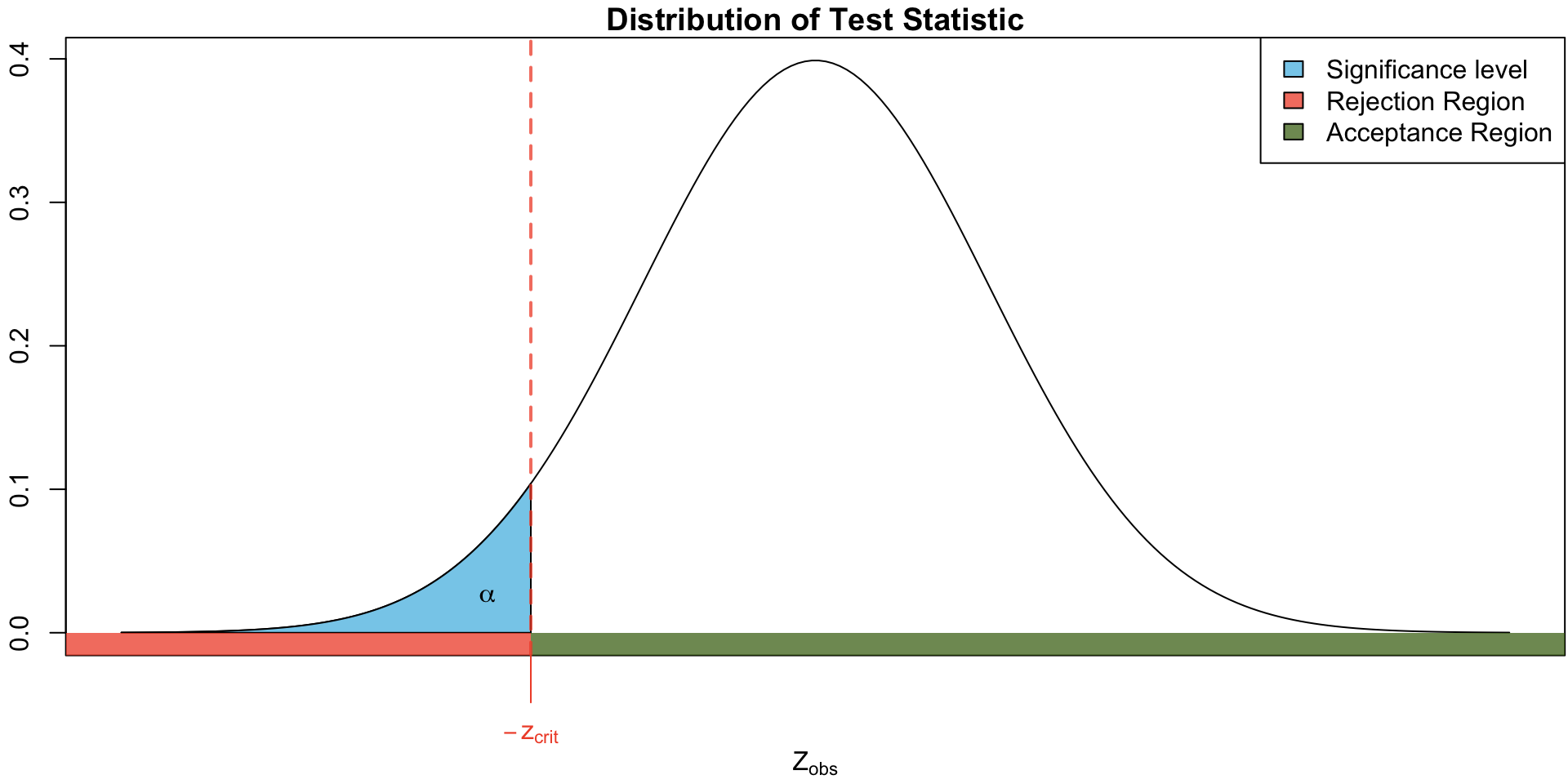
RR for lower-tail test

Critical Value approach for proportions

0. Check Assumptions. If satisfied, 1. State hypotheses \[\begin{equation} H_0 : p = p_0 \quad \text{ vs. } \quad H_A: \begin{cases} p \neq p_0& \text{ two-sided test} \\ p < p_0&\text{ one-sided (lower-tail) test} \\ p > p_0&\text{ one-sided (upper-tail) test} \end{cases} \end{equation}\]

1. Find critical value:

   \[\begin{cases} P(-z_{crit} < Z < z_{crit}) = 1 - \alpha &\text{ if } H_A: p \neq p_0 \\ P(Z < z_{crit}) = \alpha &\text{ if } H_A: p < p_0 \\ P(Z > z_{crit}) = \alpha &\text{ if } H_A: p > p_0 \end{cases}\]

2. Compute the test statistic \(z_{obs} = \dfrac{\hat p - p_0}{\sqrt{p_0(1-p_0)/n}}.\)

3. Conclusion: reject \(H_0\) if \(z_{obs} \in\) rejection region, otherwise, fail to reject \(H_0\).

Assumptions

Assumptions for Hypothesis Tests for Proportions

1. We have a simple random sample
2. The experiment can be modeled by the binomial distribution:
   • number of trials is fixed
   • trials are independent
   • only two possible outcomes (‘success’ and ‘failure’)
   • Probabilities constant for each trial
3. Success-failure condition¹: \(np \geq 10\) and \(n(1-p) \geq 10)\)

For CI \(\hat p\) is used to check the success-failure condition and compute the standard error.

For hypothesis tests, typically the null value – that is, the proportion claimed in the null hypothesis – is used in place of p.

1. Some resources only use a check of \(np \geq 5\) and \(n(1 - p) \geq 5\)

ChatGPT

Exercise 1 According to a November 2023 research survey conducted by Pew Research¹, about 13% of all U.S. teens have used the generative artificial intelligence (AI) chatbot in their schoolwork. Suppose we wish to investigate if this the proportion of students on our campus using generative AI to do homework. We survey 80 randomly selected UBCO students and find that 14 have admitted to using generative AI to do homework. Perform a formal hypothesis test for determining the proportion at UBCO differs from that of U.S. teens.

If the null was true we’d expect 10.4 of our sample of size 80 to have used generative AI for homework

1. This survey was conducted online from Sept. 26 to Oct. 23, 2023 and sampled 1,453 U.S. teens ages 13 to 17 who live with their parents by age, gender, race and ethnicity, household income, and other categories.

Check Assumption

We need to check the success-fail condition: that \(np \geq 10\) and \(n(1-p) \geq 10)\).

Important

We use the hypothesized value for these checks.

Here \(n\) = 80, our hypothesized value for \(p\) is 0.13

• \(np_0\) = 10.4 ✅

• \(np_0\) = 69.6 ✅

Solution to Exercise 1

1. State null and alternative hypotheses

   \(H_0:\)

   \(H_A:\)

2. Find the critical values:

3. Calculate the test statistic:

   \[ \begin{equation} Z_{obs} = \dfrac{\hat p - p_0}{\sqrt{p_0(1-p_0)/n}} = \end{equation} \]

4. Conclusion:

Jump ahead to corresponding Confidence Interval for p

An Alternative Test Procedure

• We now consider an alternative hypothesis-testing method for for deciding whether to reject \(H_0\).

• Like the rejection method, it will rely on a test statistic.

• Unlike the rejection method, we will no longer require a critical value, but instead calculate a certain probability that goes by the name of a \(p\)-value.

• While these two procedures should yield the same conclusion, the \(p\)-value will provide an intuitive measure of the strength of evidence in the data against \(H_0\).

P-value

\(p\)-value

Definition 1 The \(p\)-value is the probability, calculated assuming that the null hypothesis is true, of obtaining a value of the test statistic at least as contradictory to \(H_0\) as the value calculated from the available sample.

In other words, it quantifies the chances of obtaining the observed data or data more favorable to the alternative than our current data set if the null hypothesis were true.

Key points:

• The P-value is a function of the sample data.
• Calculation assumes that \(H_0\) is true.
• Let’s discuss which values of the test statistic are “at least as contradictory to \(H_0\)” as the value obtained from our sample.

Definition from Devore, Berk, and Carlton (2021) Section 9.4

\(p\)-value approach for proportions

1. State hypotheses \[\begin{equation} H_0 : p = p_0 \quad \text{ vs. } \quad H_A: \begin{cases} p \neq p_0& \text{ two-sided test} \\ p < p_0&\text{ one-sided (lower-tail) test} \\ p > p_0&\text{ one-sided (upper-tail) test} \end{cases} \end{equation}\]

2. Compute the test statistic \(z_{obs} = \dfrac{\hat p - p_0}{\sqrt{p_0(1-p_0)/n}}.\)

3. Calculate the \(p\)-value

   \[\begin{cases} 2P(Z \geq |z_{obs}|) &\text{ if } H_A: p \neq p_0 \\ P(Z \leq z_{obs}) &\text{ if } H_A: p < p_0 \\ P(Z \geq z_{obs}) &\text{ if } H_A: p > p_0 \end{cases}\]

4. Conclusion: reject \(H_0\) if \(p\)-value is less than \(\alpha\) (typically 0.05), otherwise, fail to reject \(H_0\).

Redo example using p-values

Returning to Exercise 1, and using the same hypotheses, the \(p\)-value can be calculated as follows:

\[\begin{align} 2P(Z \geq |z_{obs}|) &= 2P(Z \geq |1.1968127|) \\ &= 2 (0.1156898)\\ &= 0.2313796\\ \end{align}\]

Since this \(p\)-value = \(0.2313796\) greater than \(\alpha = 0.05\), we fail to reject \(H_0\) …

Comment

• Note that the critical value approach and the \(p\)-value approach should provide the same conclusion (provided the hypotheses, data, and significance level is the same)

• However, rather than a binary outcome (reject vs. fail to reject) the \(p\)-value gives information about the strength of evidence against the null hypothesis.

• e.g a \(p\)-value of 0.04999 and 0.0000001 are both significant, but 0.0000001 indicates stronger evidence than 0.04999.

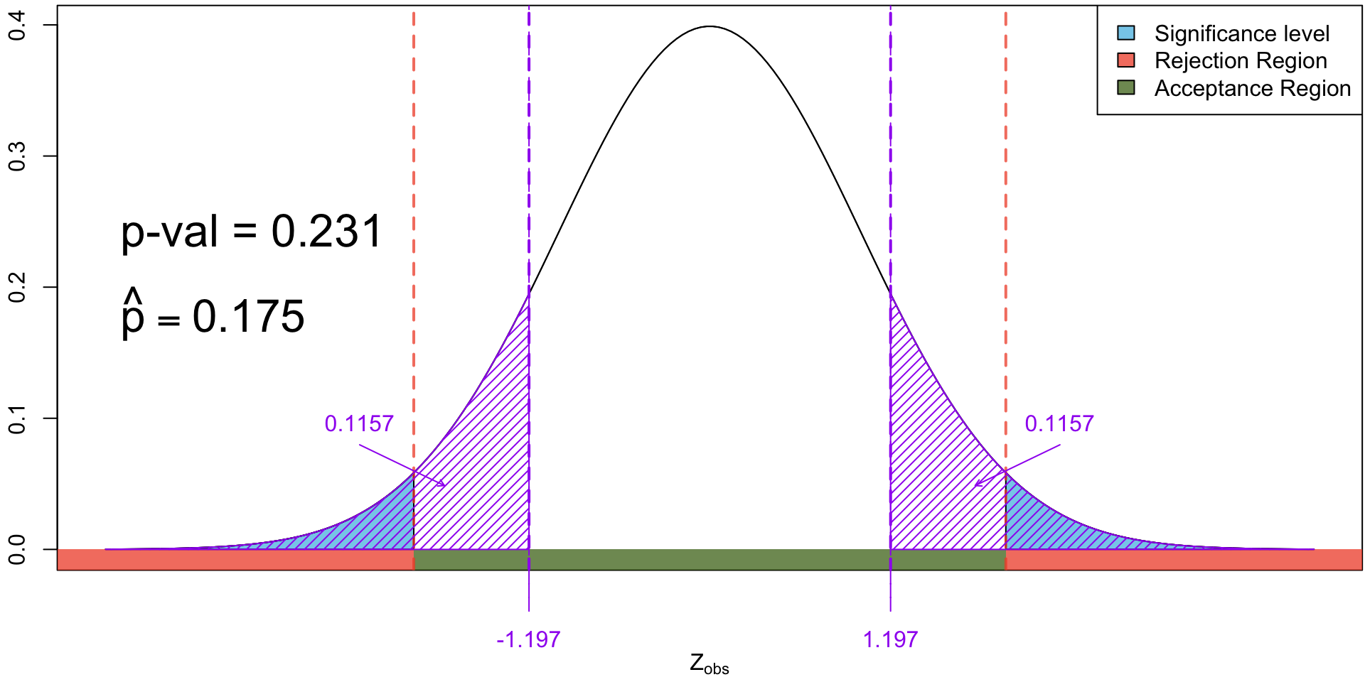
The distribution of the test statistic for testing \(H_0: p = 0.13\) vs \(H_0: p \neq 0.13\). Shaded in yellow is the \(p\)-value when we observed 14 yes’s.

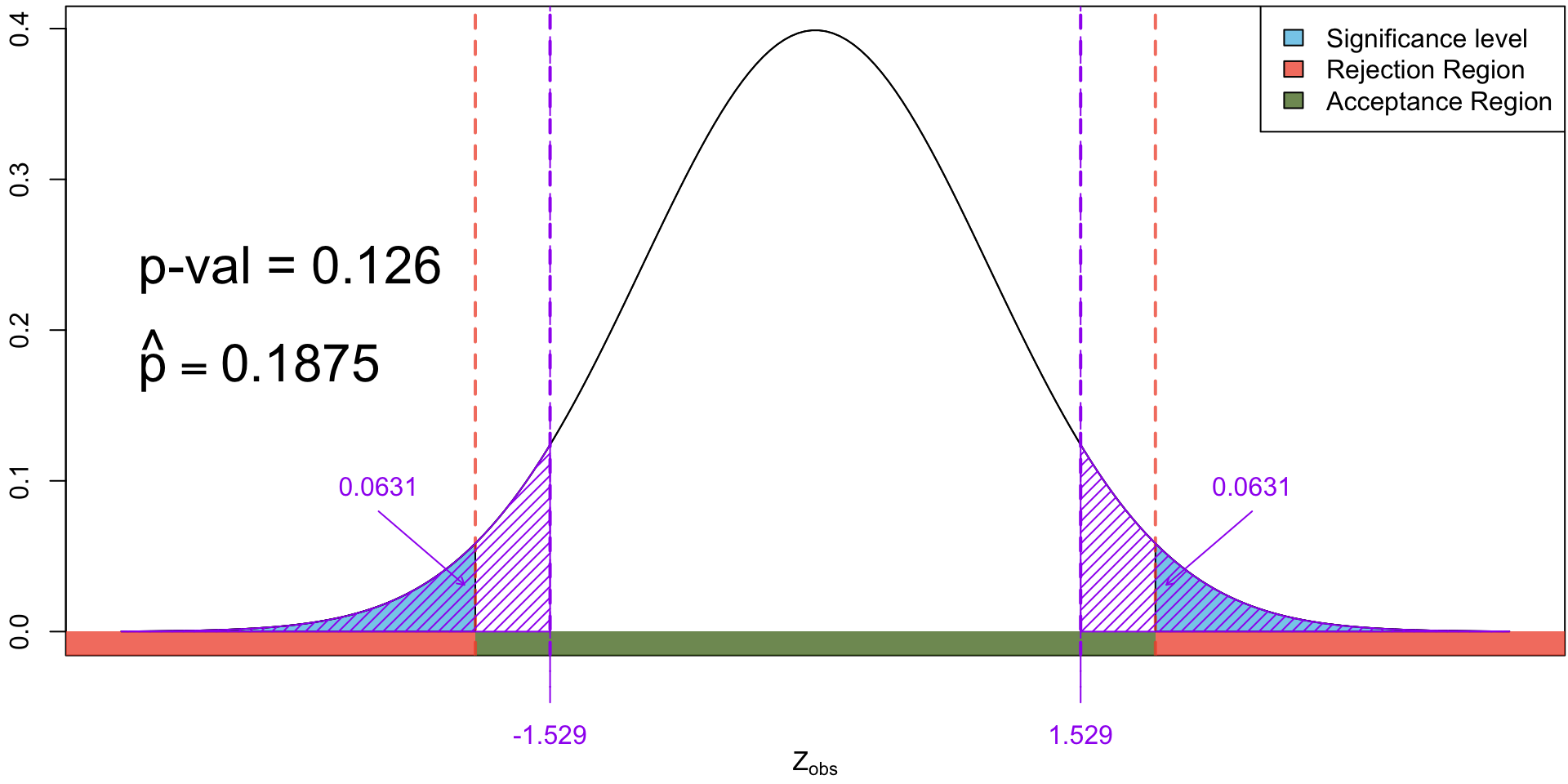
The distribution of the test statistic for testing \(H_0: p = 0.13\) vs \(H_0: p \neq 0.13\). Shaded in yellow is the \(p\)-value when we observed 15 yes’s.

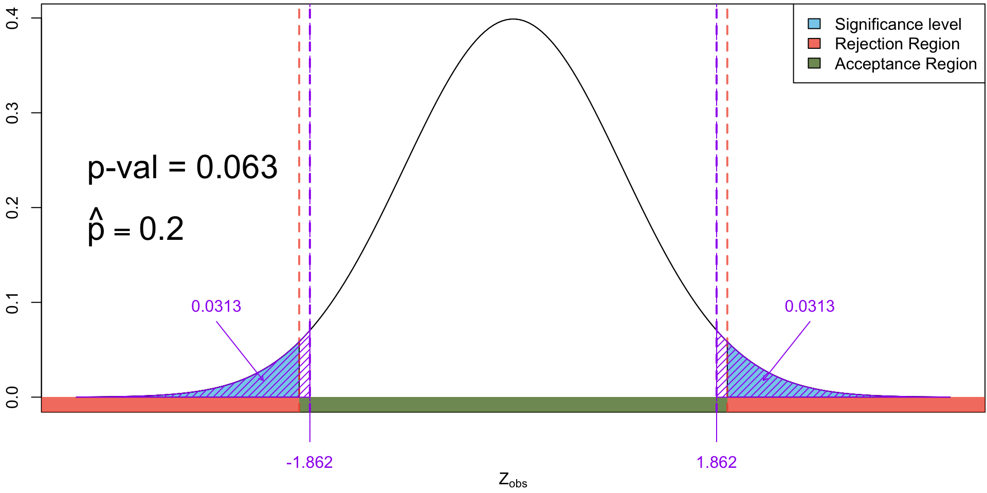
The distribution of the test statistic for testing \(H_0: p = 0.13\) vs \(H_0: p \neq 0.13\). Shaded in yellow is the \(p\)-value when we observed 16 yes’s.

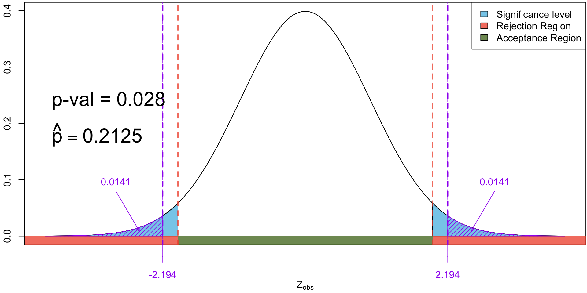
The distribution of the test statistic for testing \(H_0: p = 0.13\) vs \(H_0: p \neq 0.13\). Shaded in yellow is the \(p\)-value when we observed 17 yes’s.

The distribution of the test statistic for testing \(H_0: p = 0.13\) vs \(H_0: p \neq 0.13\). Shaded in yellow is the \(p\)-value when we observed 18 yes’s.

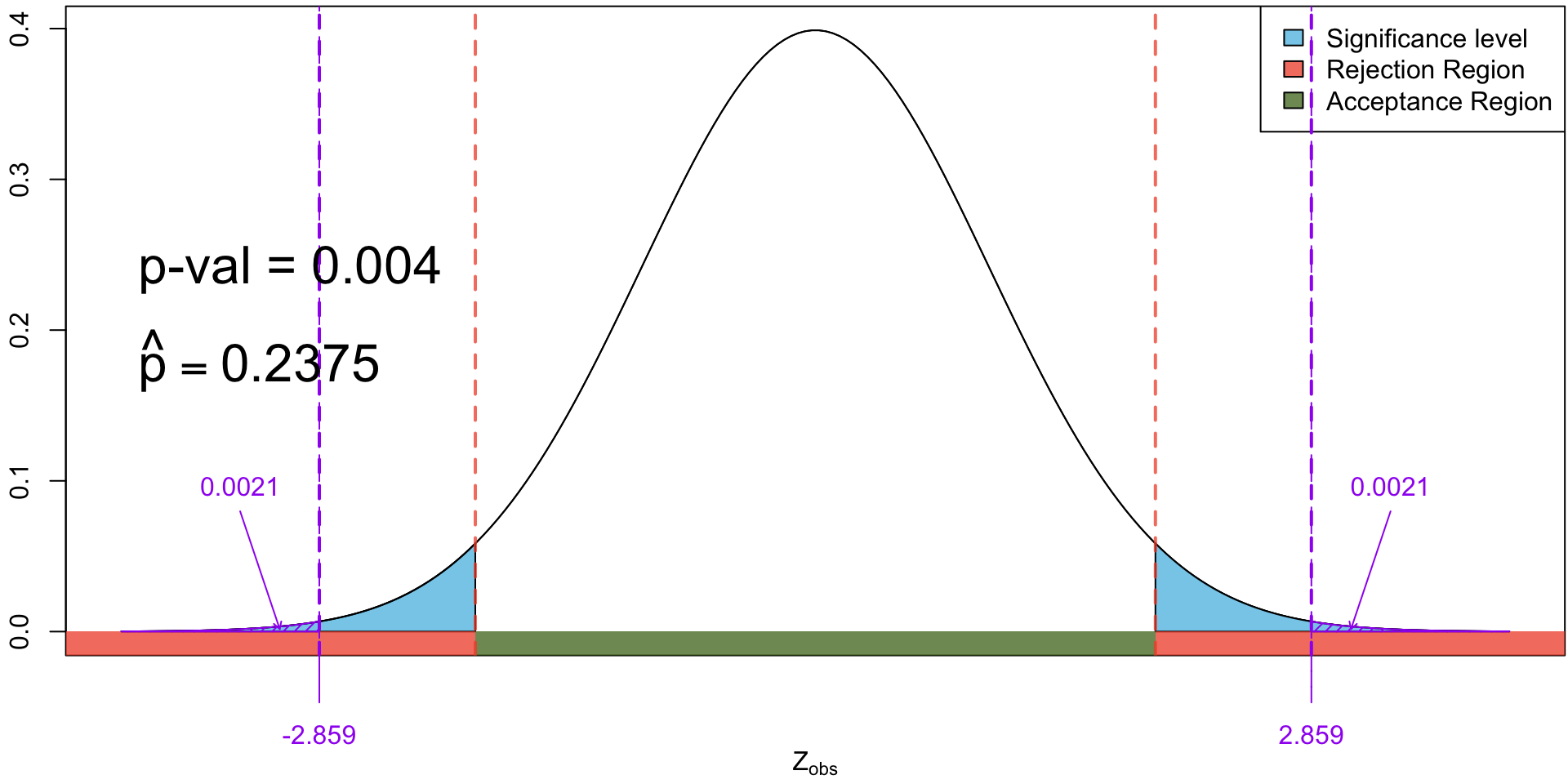
The distribution of the test statistic for testing \(H_0: p = 0.13\) vs \(H_0: p \neq 0.13\). Shaded in yellow is the \(p\)-value when we observed 19 yes’s.

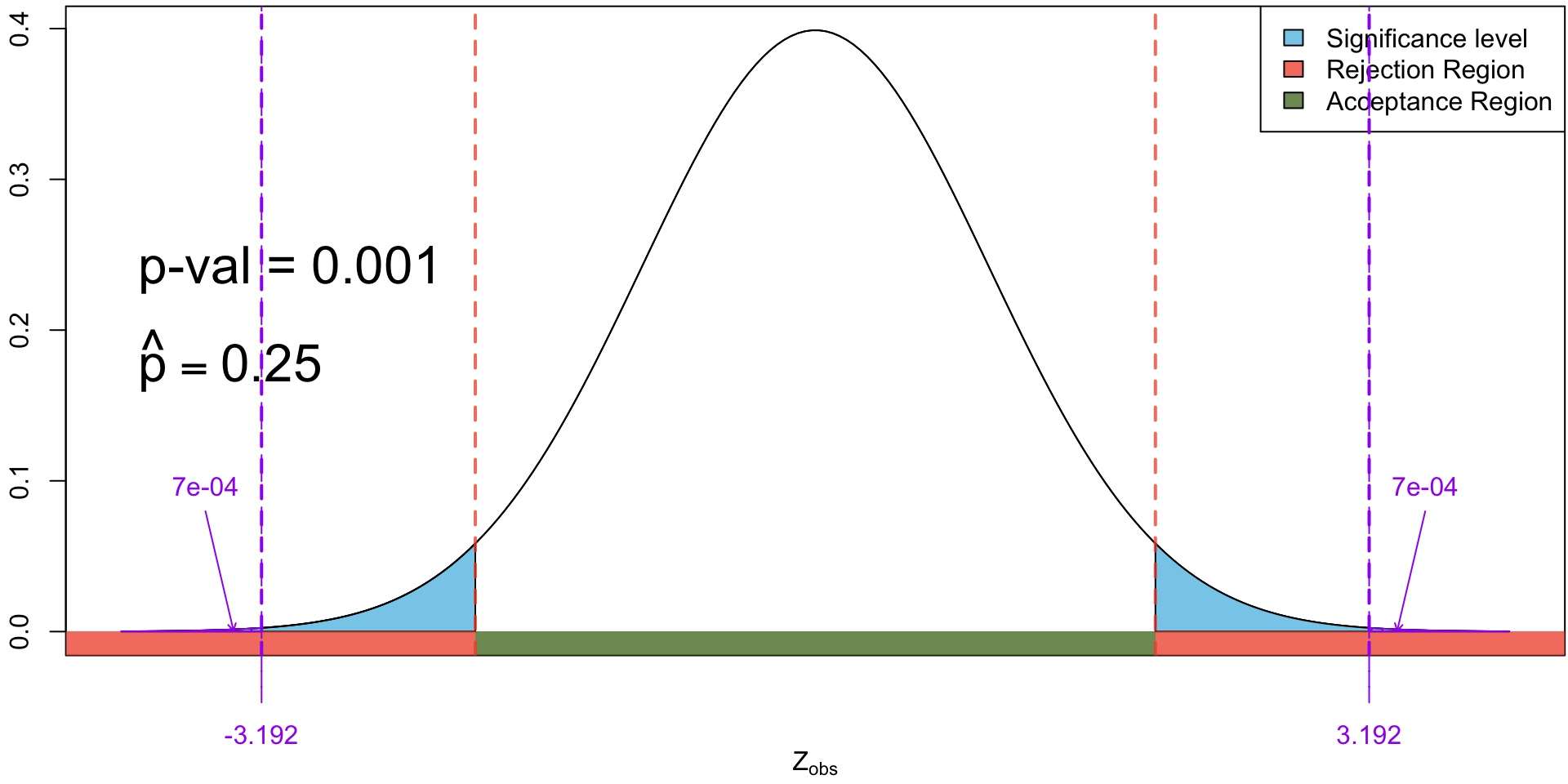
The distribution of the test statistic for testing \(H_0: p = 0.13\) vs \(H_0: p \neq 0.13\). Shaded in yellow is the \(p\)-value when we observed 20 yes’s.

Comments

When the observed test statistics falls in the rejection region, we will necessarily have a significant \(p\)-value and vice versa.

• Observing 21 out of 80 in our sample who have used generative AI for homework (i.e. \(\hat p = \frac{21}{80}\) = 0.2625) yields a very small \(p\)-value (<0.001). Hence we have very strong evidence against the null hypothesis \(H_0\).
• 17 out of 80 (i.e. \(\hat p = \frac{17}{n}\) = 0.2125 ) yields a significant \(p\)-value (0.028), but evidence is not as strong as a sample with 20 “yes”s.
• 16 out of 80 (i.e. \(\hat p = \frac{16}{80}\) = 0.2) yields an almost significant \(p\)-value (0.063). Hence we have insufficient evidence against \(H_0\) but may still have our suspicions.

Recall the \(p_0\) = 0.13

Interpreting \(p\)-values

Here are some guidelines for using the \(p\)-value to assess the evidence against the null hypothesis at \(\alpha = 0.05\).

\(p\)-value	Evidence against \(H_0\)	Significance code in R
\(0.1 \leq p \leq 1\)	no evidence
\(0.05 < p \leq 0.10\)	weak evidence	.
\(0.01 < p \leq 0.05\)	sufficient evidence	*
\(0.001 < p \leq 0.01\)	strong evidence	**
\(0< p \leq 0.001\)	very strong evidence	***

Notice how we don’t have this probabilistic interpretation when using the critical value method.

Battery Life of a New Smartphone 📱🔋

Exercise 2 A smartphone company advertises that their new model lasts an average of 20 hours per charge under normal usage. A tech reviewer, skeptical of the claim, decides to test whether the battery actually lasts less than 20 hours on average. They collect a random sample of 40 phones and observe an average battery life of 19.66 hours. Assuming \(\sigma = 1.2\) and a significance level of \(\alpha = 0.05\), test whether the phone’s battery life is significantly less than the advertised 20 hours.

Lower-tailed test

Hypotheses

\[ \begin{align} H_0:& \mu = 20 & H_1: &\mu < 20 \end{align} \]

Test Statistic

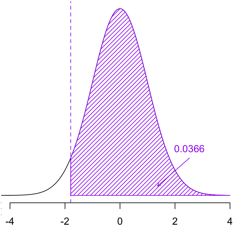
\[ \begin{align} z_{obs} &= \frac{\bar x - \mu_0}{\sigma/\sqrt{n}} = \frac{19.66 - 20}{1.2/\sqrt{40}} = -1.7919573 \end{align} \] \(p\)-value

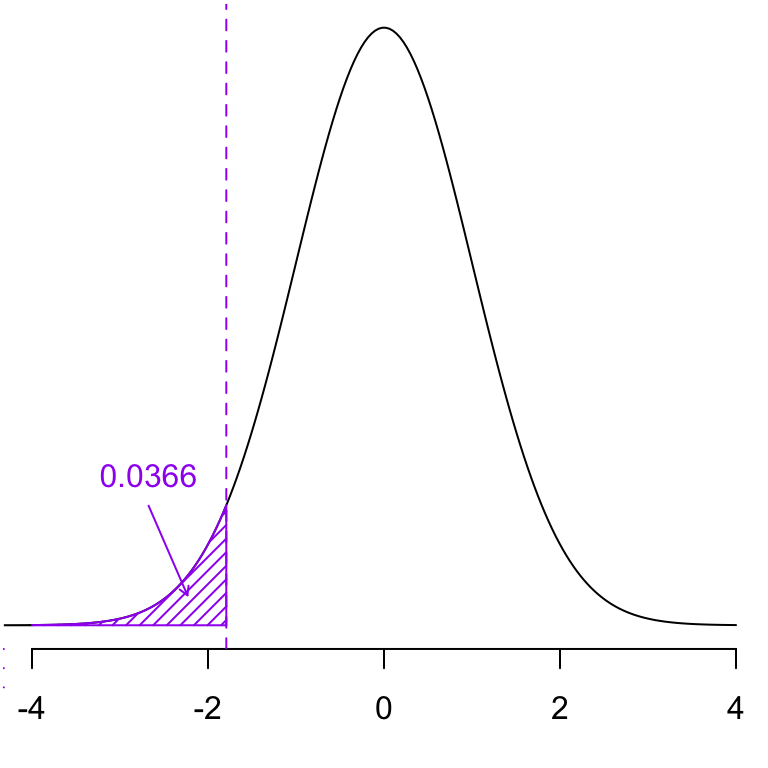
\[ \begin{align*} \Pr(Z \leq z_{obs}) = \Pr(Z \leq -1.79) \approx 0.0366 \end{align*} \] Conclusion

Since the \(p\)-value \(< \alpha\) we reject \(H_0\) in favour of the alternative. Hence, there is statistically significant evidence to suggest that the average battery life for this model of smartphone is less than the advertised 20 hours.

Lower Tailed

\[ \begin{align} H_0:& \mu = 20 & H_1: &\mu < 20 \end{align} \]

\(z_{obs} = -1.7919573\)

\(p\)-value \[ \begin{align} &= \Pr(Z \leq z_{obs}) \\ &= \Pr(Z \leq -1.79) \\ & \approx 0.0366 \end{align} \]

Reject \(H_0\)

Upper Tailed

\[ \begin{align} H_0:& \mu = 20 & H_1: &\mu \textcolor{red}{>} 20 \end{align} \]

\(z_{obs} = -1.7919573\)

\(p\)-value \[ \begin{align} &= \Pr(Z \textcolor{red}{\geq} z_{obs}) \\ &= \Pr(Z \textcolor{red}{\geq} -1.79) \\ & \approx \textcolor{red}{0.9634} \end{align} \]

\(\textcolor{red}{\text{Fail to}}\) reject \(H_0\)

Two-Tailed

\[ \begin{align} H_0:& \mu = 20 & H_1: &\mu \textcolor{red}{\neq} 20 \end{align} \]

\(z_{obs} = -1.7919573\)

\(p\)-value \[ \begin{align} &= \textcolor{red}{2 \times}\Pr(Z \textcolor{red}{\geq} \textcolor{red}{|z_{obs}|}) \\ &= \textcolor{red}{2 \times}\Pr(Z \textcolor{red}{\geq} \textcolor{red}{1.79}) \\ & \approx \textcolor{red}{0.0731} \end{align} \]

\(\textcolor{red}{\text{Fail to}}\) reject \(H_0\)

Jump ahead to corresponding Confidence Interval

iClicker

Connection with p-values and null distributions

If the null hypothesis is false, the \(p\)-value of a hypothesis test at \(\alpha = 0.05\) will be less than 0.05 in which of the following cases?

1. Always
2. Never
3. Sometimes

Connection with Confidence Intervals

Suppose we find a (1-\(\alpha\))100% confidence interval for \(\mu\) using:

\[ \begin{align} \bar x \pm z_{\alpha/2} \frac{\sigma}{\sqrt{n}} \end{align} \]

And we wish to carry out a test of:

\[ \begin{align} H_0&: \mu = \mu_0 & H_A&: \mu = \mu_0 \end{align} \]

with a significance level of \(\alpha\)…

Steps in formal hypothesis test

To answer this we would usually calculate our test statistic:

\[ Z_{obs} = \dfrac{\bar X - \mu_0}{\sigma/\sqrt{n}} \]

and check if it falls into the rejection region, or alternatively, calculate the corresponding \(p\)-value and compare it with \(\alpha\).

Alternatively, I could tell you the decision of that test by looking at the confidence interval….

Connection between Confidence Intervals and Two-Sided Hypothesis Tests

Consider a two-sided hypothesis test at a significance level of \(\alpha\)

\[ \begin{align} H_0&: \mu = \mu_0 & H_A&: \mu \neq \mu_0 \end{align} \]

Suppose we construct the (1- \(\alpha\))% confidence interval (CI) for \(\mu\), using

\[ \begin{align} \bar x \pm z_{\alpha/2} \frac{\sigma}{\sqrt{n}} \end{align} \]

Test Procedure:

• If the \(\mu_0\) falls within the CI, we do not have sufficient evidence to reject \(H_0\).

• If the \(\mu_0\) falls outside the CI, we have sufficient evidence to reject \(H_0\).

will be comprised of all values of \(\mu_0\) for which we would not reject the null hypothesis.

Confidence Interval

Returning to the Two sided Test, let’s find the corresponding 95% CI:

\[ \begin{align} \bar x &\pm z_{\alpha/2} \frac{\sigma}{\sqrt{n}}\\ 19.66 &\pm \frac{1.2}{\sqrt{40}}\\ 19.66 &\pm 0.371877 \\ [19.29&, 20.03] \end{align} \]

Since \(\mu_0 = 20\) falls within the 95% CI, we have insufficient evidence to reject the null hypothesis.

Confidence Interval for p

Returning to Exercise 1, a 95% CI based on 14 out of 80 “yes”s.

\[ \begin{align} \hat p &\pm z_{\alpha/2} \sqrt{\frac{p_0(1-p_0)}{n}}\\ 0.175 &\pm 1.96 \frac{0.13(1- 0.13)}{\sqrt{80}}\\ 0.175 &\pm 0.07369574 \\ [0.1013&, 0.2487] \end{align} \]

Since \(p_0\) = 0.13 lies within this CI we would fail to reject the null hypothesis that \(p = 0.13\)

note how the standard error is calculated assuming the null hypothesis.

Confidence Interval for p

Returning to Exercise 1, a 95% CI based on 17 out of 80 “yes”s.

\[ \begin{align} \hat p &\pm z_{\alpha/2} \sqrt{\frac{p_0(1-p_0)}{n}}\\ 0.2125 &\pm 1.96 \frac{0.13(1- 0.13)}{\sqrt{80}}\\ 0.2125 &\pm 0.07369574 \\ [0.1388&, 0.2862] \end{align} \]

Since \(p_0\) = 0.13 does not lie within this CI would have sufficient evidence to reject the null hypothesis that \(p = 0.13\)

iClicker

Connection with p-values and CI

The \(p\)-value for a two-sided hypothesis test of \(H_0: \mu = \mu_0\) is found to be 0.021. Would a 95% confidence interval for \(\mu\) contain \(\mu_0\)

1. Yes
2. No
3. There is not enough information to say

iClicker

Connection with p-values and CIs

The \(p\)-value for a two-sided hypothesis test of \(H_0: \mu = \mu_0\) is found to be 0.021. Would a 99% confidence interval for \(\mu\) contain \(\mu_0\)

1. Yes
2. No
3. There is not enough information to say

Resources

Devore, J. L., K. N. Berk, and M. A. Carlton. 2021. Modern Mathematical Statistics with Applications. Springer Texts in Statistics. Springer International Publishing. https://books.google.ca/books?id=ghcsEAAAQBAJ.