Chi-squared Tests

STAT 205: Introduction to Mathematical Statistics

Dr. Irene Vrbik

University of British Columbia Okanagan

Outline

• Chi-squared tests, as it’s name suggests, are a family of statistical hypothesis tests that rely on the Chi-squared distribution.

• Chi-squared tests are used to determine whether there’s a significant difference between observed and expected frequencies in categorical data.

• Goal: Understand when and how to use different types of chi-squared tests.

It is pronounced “kai” (as in kite)

Types of Chi-squared tests

Goodness-of-Fit

Test of Independence

Test of Homogeneity

• One categorical variable
• One group

• 2 categorical variables
• One group

• One categorical variable
• Multiple groups

e.g. M&M colors evenly distributed?

e.g. Is gender related to music streaming preference?

e.g. Do different schools have the same music streaming preferences?

All three tests can be framed as special cases of contingency table analysis.

There are three main types:

Goodness-of-fit tests: Does the distribution of categories match a known distribution?

Are the distributions of a single variable the same across groups?

Test of Independence: Are the two variables associated (i.e., dependent)?

Independence test → random sample from one population

Homogeneity test → samples from multiple populations

• One-Way

• Two-Way

Goodness-of-Fit

🟢	🔵	🟡	🟠	🟤	🔴
48	51	46	52	49	54

Independence

female	90	110	50
male	110	70	70
other	30	20	10

Homogeneity

UBC	150	30	20
UofT	120	50	30
McGill	130	40	30

\[ \underbrace{\rule{15em}{0pt}}_{\text{One Population}} \]

\[ \underbrace{\rule{8em}{0pt}}_{\text{Three Populations}} \]

if M&Ms were uniformly distributed, we’d expect a roughly similar amount of M&Ms for each colour

One-way Contingency Table

• A contingency table¹ presents the frequency distribution of variables in a matrix format.

• A one-way table is simplye a frequency table for a single categorical variable.

  🟢	🔵	🟡	🟠	🟤	🔴
  48	51	46	52	49	54

See this post on how to create contingency tables in R.

1. also known as a cross-tabulation or crosstab or two-way table.

Two-way Table

• A two-way table displays the joint distribution of two categorical variables.

• The rows represent the categories of one variable, while the columns represent the categories of another.

\(\quad\quad\quad\quad\quad\quad\overbrace{\phantom{\rule{8em}{0pt}}}^{\text{Variable 2}}\)

\[ \text{Variable 1} \begin{cases} \text{}\\ \text{}\\ \text{}\\ \end{cases} \]

Female
Male
Other

• Contingency Table Analysis can be used to analyze the relationship between one or two categorical variables.

• It is often used to understand if the variables are independent of each other or if there is a significant association between them.

• This analysis is fundamental in various fields such as epidemiology, marketing, sociology, and psychology.

Two-way Table

	Spotify	Apple Music	Youtube Music
Female
Male		cell
Other

A cell displays the count for the intersection of a row and column.

Two-way Table

	Spotify	Apple Music	YouTube Music
female	90	110	50
male	110	70	70
other	30	20	10

For example, 70 other people we surveyed we male and preferred Apple Music for streaming music

Marginal Totals

	Spotify	Apple Music	YouTube Music	Row Total
female	90	110	50	250
male	110	70	70	250
other	30	20	10	60
Col Total	230	200	130	560

- Marginal Totals: The total observations in the respective row/column are usually provided in the margins

- The total observation count is given in the bottom right-hand corner

Contingency Tables

	Level 1	Level 2	Total
Group A	\(A\)	\(B\)	\(A + B\)
Group B	\(C\)	\(D\)	\(C + D\)
Total	\(A +C\)	\(B + D\)	\(T\)

• \(A, B, C, D\): Number of observations for a specific category combination.

• The marginal totals are given in the marigns, and represent the total observations in the respective row/column.
• \(T = A+ B+ C+D\): Total observations in the table.

The primary method for displaying the summarization of categorical variables is called a contingency table.

When we have two measurements on our subjects that are both categorical, the contingency table is sometimes referred to as a two-way table.

“two-way” terminology: because the table consists of rows and columns (i.e., the data display goes two ways).

Each cell shows the count (or proportion) of observations falling into that combination of variable levels.

Goodness-of-Fit test

aka One-Way Chi-squared tests

Hypotheses

🎨 Example 1: M&M Colors (Uniform Distribution)

• \(H_0\): The colours of M&Ms are equally distributed (each color appears with the same probability).

• \(H_A\): The colours of M&Ms are not equally distributed.

\(H_0\): The proportion of each M&M color in the population is:

\[ p_\text{green} = p_\text{blue} = p_\text{yellow} = p_\text{orange} = p_\text{brown} = p_\text{red} = \frac{1}{6} \]

\(H_A\): At least one of the color proportions is not equal to \(\frac{1}{6}\)

Chi-squared Test Statistic

• Chi-squared tests determine if there’s a statistically significance by comparing observed frequencies to expected frequencies under the null hypothesis.

• For example, if assume that M&M colours are evenly distributed we would expect the proportion of each colour to be the same.

• In terms of counts, if our M&M container contained 300 M&Ms we would expect there to be 300/6 = 50 M&Ms of each colour.

Expected vs Observed M&M counts

Observed M&M counts

🟢	🔵	🟡	🟠	🟤	🔴
48	51	46	52	49	54

Expected M&M counts

🟢	🔵	🟡	🟠	🟤	🔴
50	50	50	50	50	50

Is this difference in expected vs observed counts enough to make us question hypothesized distribution?

Chi-squared test statistic

When the observed counts are close to the expected, this test stat will be small

The chi-squared test statistic measures the difference between observed and expected counts:

\[ \chi^2 = \sum \dfrac{(\text{Observed} - \text{Expected})^2}{\text{Expected}} \]

For a one-way chi-square (aka goodness of fit) test, this test statistic follows a Chi-squared distribution with degrees of freedom equal to the number of categories minus 1 (\(k- 1\))

df = number of cells in our contigency table -1

M&Ms Observed Test Stat

Observed M&M counts

🟢	🔵	🟡	🟠	🟤	🔴
48	51	46	52	49	54

Expected M&M counts

🟢	🔵	🟡	🟠	🟤	🔴
50	50	50	50	50	50

\[ \begin{align} \chi^2 &= \dfrac{48 - 50}{50} \phantom{+ \dfrac{51 - 50}{50} + \dfrac{46 - 50}{50} + \dots} \\ \phantom{\dots} & \phantom{+ \dfrac{52 - 50}{50} + \dfrac{49 - 50}{50} + \dfrac{54 - 50}{50}}\\ &\phantom{= } \end{align} \]

M&Ms Observed Test Stat

Observed M&M counts

🟢	🔵	🟡	🟠	🟤	🔴
48	51	46	52	49	54

Expected M&M counts

🟢	🔵	🟡	🟠	🟤	🔴
50	50	50	50	50	50

\[ \begin{align} \chi^2 &= \dfrac{48 - 50}{50} + \dfrac{51 - 50}{50} \phantom{+ \dfrac{46 - 50}{50} + \dots} \\ \phantom{\dots} & \phantom{+ \dfrac{52 - 50}{50} + \dfrac{49 - 50}{50} + \dfrac{54 - 50}{50}}\\ &\phantom{= } \end{align} \]

M&Ms Observed Test Stat

Observed M&M counts

🟢	🔵	🟡	🟠	🟤	🔴
48	51	46	52	49	54

Expected M&M counts

🟢	🔵	🟡	🟠	🟤	🔴
50	50	50	50	50	50

\[ \begin{align} \chi^2 &= \dfrac{48 - 50}{50} + \dfrac{51 - 50}{50} + \dfrac{46 - 50}{50} \phantom{+ \dots} \\ \phantom{\dots} & \phantom{+ \dfrac{52 - 50}{50} + \dfrac{49 - 50}{50} + \dfrac{54 - 50}{50}}\\ &\phantom{= } \end{align} \]

M&Ms Observed Test Stat

Observed M&M counts

🟢	🔵	🟡	🟠	🟤	🔴
48	51	46	52	49	54

Expected M&M counts

🟢	🔵	🟡	🟠	🟤	🔴
50	50	50	50	50	50

\[ \begin{align} \chi^2 &= \dfrac{48 - 50}{50} + \dfrac{51 - 50}{50} + \dfrac{46 - 50}{50} + \dots \\ \dots & + \dfrac{52 - 50}{50} \phantom{+ \dfrac{49 - 50}{50} + \dfrac{54 - 50}{50}}\\ &\phantom{= } \end{align} \]

M&Ms Observed Test Stat

Observed M&M counts

🟢	🔵	🟡	🟠	🟤	🔴
48	51	46	52	49	54

Expected M&M counts

🟢	🔵	🟡	🟠	🟤	🔴
50	50	50	50	50	50

\[ \begin{align} \chi_{obs}^2 &= \dfrac{48 - 50}{50} + \dfrac{51 - 50}{50} + \dfrac{46 - 50}{50} + \dots \\ \dots & + \dfrac{52 - 50}{50} + \dfrac{49 - 50}{50} + \phantom{\dfrac{54 - 50}{50}}\\ &\phantom{= } \end{align} \]

M&Ms Observed Test Stat

Observed M&M counts

🟢	🔵	🟡	🟠	🟤	🔴
48	51	46	52	49	54

Expected M&M counts

🟢	🔵	🟡	🟠	🟤	🔴
50	50	50	50	50	50

\[ \begin{align} \chi^2 &= \dfrac{48 - 50}{50} + \dfrac{51 - 50}{50} + \dfrac{46 - 50}{50} + \dots \\ \dots & + \dfrac{52 - 50}{50} + \dfrac{49 - 50}{50} + \dfrac{54 - 50}{50}\\ &\phantom{= } \end{align} \]

M&Ms Observed Test Stat

Observed M&M counts

🟢	🔵	🟡	🟠	🟤	🔴
48	51	46	52	49	54

Expected M&M counts

🟢	🔵	🟡	🟠	🟤	🔴
50	50	50	50	50	50

\[ \begin{align} \chi^2 &= \dfrac{48 - 50}{50} + \dfrac{51 - 50}{50} + \dfrac{46 - 50}{50} + \dots \\ \dots & + \dfrac{52 - 50}{50} + \dfrac{49 - 50}{50} + \dfrac{54 - 50}{50}\\ & = \boxed{0.84} \end{align} \]

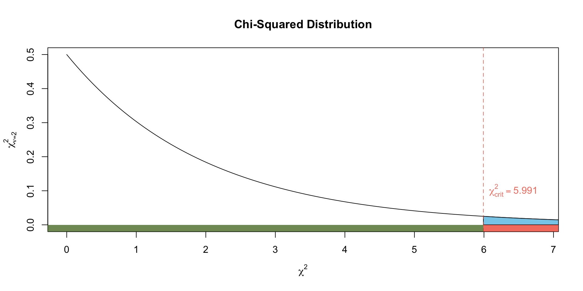
Rejection Region

Figure 1: Illustrates the Rejection Region on a Chi-squared distribution with 5 degrees of freedom

p-value

Figure 2: Illustrates the \(p\)-value associated with our observed test statistic on our null chi-squared distribution with 5 degrees of freedom

iClicker

Chi-squared \(p\)-value

Exercise 1 (M&M p-value) How would we calculate the \(p\)-value in R?

1. pnorm(0.84, lower.tail = FALSE)

2. pchisq(0.05, df = 5, lower.tail = FALSE)

3. qchisq(0.84, df = 5, lower.tail = FALSE)

4. pchisq(0.84, df = 5, lower.tail = FALSE)

5. None of the above

Conclusion

• Since the \(p\)-value is greater than our significance level (\(\alpha = 0.05\)) we would fail to reject the null hypothesis.

• Hence, there is insufficient evidence to suggest that the M&Ms are not uniformly distributed in color.

• Equivalently, there is no statistical evidence to suggest that the proportions of M&Ms differ by colour.

Comment

• When we only have two levels (aka categories) for our categorical variable the Chi-square goodness-of-fit test is equivalent¹ to the one-sample \(Z\)-test for proportions².

• However, the Z-test only works for one proportion at a time (e.g., is the proportion of heads = 0.5?).

• The Chi-Square test is more flexible and can handle multiple categories simultaneously.

1. they are testing the same thing and yield the same \(p\)-value. The test statistics have the relationship of \(\chi_{obs}^2 = Z_{obs}^2\)

2. for more details see this YouTube video.

Test for Independence

aka Two-Way Chi-Square Test

Probabilities from tables

	Success	Failure	Total
Group 1	\(A\)	\(B\)	\(A + B\)
Group 2	\(C\)	\(D\)	\(C + D\)
Total	\(A +C\)	\(B + D\)	\(T\)

For example:

Let \(G_1\) denote the event of belonging to ‘Group 1’

Let \(S\) denote the event ‘Success.’

\[\begin{align} \Pr(G_1) &= \dfrac{A+B}{T} & \Pr(S) &= \dfrac{A+C}{T} \end{align}\]

Independence

Recall that if two events are independent, then their intersection is the product of their respective probabilities.

\[\begin{align} \Pr(A \cap B) &= \Pr(A) \Pr(B) \end{align}\]

In our case, if \(G_1\) and \(S\) are idependent we would expect: \[\begin{align} \Pr(G_1 \cap S) &= \dfrac{A+B}{A+B+C+D}* \dfrac{A+C}{A+B+C+D} \\ &= \dfrac{(A+B)(A+C)}{(A+B+C+D)^2}\\ \end{align}\]

Expected Counts

To convert to an expected count, multiple the probability (which was calculated assuming independence) by the total sample size:

\[ \dfrac{(A+B)(A+C)}{(A+B+C+D)^2} \times T\\ \]

\[ \dfrac{(A+B)(A+C)}{T^2} \times T\\ \]

\[ \dfrac{(A+B)(A+C)}{T} \]

Expected Counts Table

We can calculate the expected counts in each cell:

	Success	Failure	Total
Group A	\(\frac{(A+B)(A+C)}{T}\)	\(\frac{(A+B)(B+D)}{T}\)	\(A + B\)
Group B	\(\frac{(C+D)(A+C)}{T}\)	\(\frac{(C+D)(B+D)}{T}\)	\(C + D\)
Total	\(A +C\)	\(B + D\)	\(T\)

Expected cell count

The expected count for each cell under the null hypothesis is:

\[ \dfrac{(\text{row total})(\text{column total})}{(\text{total sample size})} \]

Example

Political Affiliation and Opinion Section

Exercise 2 A random sample of 500 U.S. adults is questioned regarding their political affiliation and opinion on a tax reform bill. The results of this survey are summarized in the following contingency table:

	Favor	Indifferent	Opposed	Total
Democrat	138	83	64	285
Republican	64	67	84	215
Total	202	150	148	500

We want to determine if an association (relationship) exists between Political Party Affiliation and Opinion on Tax Reform Bill. That is, are the two variables dependent?

Don’t include the ‘total’ row and a ‘total’ column (which represent the marginal totals)

Key Concepts

Independence: Variables are independent if the distribution of one variable is the same for all categories of the other.

Association/Dependence: If variables are not independent (i.e dependent), they may have an association.

In Exercise 2: If political affiliation is independent of opinion on a tax reform bill, this implies that the proportion of Democrats and Republicans who favor, are indifferent to, or oppose the bill should be roughly the same, reflecting no preference trend influenced by their political group.

The strength and direction of this association can be measured with various statistics, such as Phi coefficient, Cramer’s V, or the odds ratio.

Hypotheses

There are several ways to phrase these hypotheses including:

Null Hypothesis (\(H_0\))

In the population, …

1. the two categorical variables are independent
2. there is no association between the two categorical variables.
3. there is no relationship between the two categorical variables

Alternative Hypothesis (\(H_A\))

In the population, …

1. the two categorical variables are dependent
2. there is an association between the two categorical variables.
3. there is a relationship between the two categorical variables

“there is no relationship between the two categorical variables” versus “there is a relationship between the two categorical variables.

Observed Counts Table

The Observed Counts Table (or simply Observed Table) represents the observed counts obtained from our sample.

	Favor	Indifferent	Opposed	Total
Democrat	138	83	64	285
Republican	64	67	84	215
Total	202	150	148	500

In proportions you will discover that in the expected table each opinion proportion is the same for democrats and republicans. That is, from the expected counts, 0.404 of the democrats and 0.404 of the republicans favor the bill; 0.3 of the democrats and 0.3 of the republicans are indifferent; and 0.296 of the democrats and 0.296 of the republicans are opposed.

Expected Counts Table

This table represents the expected counts under the null hypothesis, i.e., the frequency of observations that would be expected if the two variables (political affiliation and opinion) were independent.

	Favor	Indifferent	Opposed	Total
Democrat	\(\frac{285\cdot 202}{500} = 115.14\)	\(\frac{285\cdot 150}{500} = 85.5\)	\(\frac{285\cdot 148}{500} = 84.36\)	285
Republican	\(\frac{215\cdot 202}{500} = 86.86\)	\(\frac{215\cdot 150}{500} = 64.5\)	\(\frac{215\cdot 148}{500} = 63.64\)	215
Total	202	150	148	500

If independent

we would be saying that the sample counts should show similarity in opinions of tax reform between democrats and republicans.

If you find the proportion of each cell by taking a cell’s expected count divided by its row total, you will discover that in the expected table each opinion proportion is the same for democrats and republicans.

That is, from the expected counts, 0.404 of the democrats and 0.404 of the republicans favor the bill; 0.3 of the democrats and 0.3 of the republicans are indifferent; and 0.296 of the democrats and 0.296 of the republicans are opposed.

Proportions

The Observed Proportions: the proportion of each cell by taking a cell’s observed count divided by its row total

	Favor	Indifferent	Opposed	Total
Democrat	0.48	0.29	0.22	0.57
Republican	0.3	0.31	0.39	0.43
Total	0.404	0.3	0.296	1

The Expected proportions: the proportion of each cell by taking a cell’s expected count divided by its row total

	Favor	Indifferent	Opposed	Total
Democrat	0.404	0.3	0.296	0.57
Republican	0.404	0.3	0.296	0.43
Total	0.404	0.3	0.296	1

🤔 Question: Is it reasonable to conclude the difference between the observed and expected counts are merely a result of random chance, or is there exists substantial evidence to question our null hypothesis.

“Are the differences between what we observed and what we expected just due to random chance, or are they too big to ignore?”

Test Statistic

Chi-Square Test Statistic

• In a summary table, we have \(r \times c = rc\) cells
• Let \(O_i\) denote the observed counts for the \(i\)th cell and
• let \(E_i\) denote the expected counts for the \(i\)th cell.

The Chi-square test statistic measures the difference between observed and expected frequencies. Under the null hypothesis, the test statistics will have (approximately) a chi-squared distribution with degrees of freedom \((r-1)(c - 1)\).

\[ \begin{equation} \chi^{2} = \sum_{i = 1}^{rc} \dfrac{(O_i - E_i)^2}{E_i} \end{equation} \]

Comments on the Test Statistic

• When the observed counts are close the expected counts, our test statistic will be small.

• Conversely, if there’s a big difference between the observed and expected counts, the test statistic will be large.

• Hence a higher test statistic value implies stronger evidence against the null hypothesis (i.e., smaller \(p\)-values).

We will summarize the strength of the evidence against the null hypothesis with a \(p\)-value

Assumptions

Conditions for the chi-square test

There are two conditions that must be checked before performing a chi-square test:

1. Independence. Each case that contributes a count to the table must be independent of all the other cases in the table.
2. Sample size / distribution. Each particular scenario (i.e. cell count) must have at least 5 expected cases.

Failing to check conditions may affect the test’s error rates.

Observed Test Statistic

The Observed Counts Table

	Favor	Indifferent	Opposed	Total
Democrat	138	83	64	285
Republican	64	67	84	215
Total	202	150	148	500

The Expected Counts Table

	Favor	Indifferent	Opposed	Total
Democrat	115.14	85.5	84.36	285
Republican	86.86	64.5	63.64	215
Total	202	150	148	500

\[ \begin{align} \chi^{2}_{obs} &= \frac{(138 - 115.14)^2}{115.14} + \frac{(83 - 115.14)^2}{85.5} + \frac{(64 - 115.14)^2}{84.36} + \dots \\ & \quad \dots \frac{(64 - 115.14)^2}{86.86} + \frac{(67 - 115.14)^2}{64.5} + \frac{(84 - 115.14)^2}{84.36} \\ &= 22.1524686 \end{align} \]

We now compare this to a chi-square distribution with \((r-1)(c-1)\) = \((2-1)*(3-1)\) = 2 degrees of freedom.

Critical Value

As we have done with other statistical tests, we make our decision by either comparing the value of the test statistic to a critical value (rejection region approach) or by finding the probability of getting this test statistic value or one more extreme (p-value approach).

Decision

Using a df of \((r-1)(c-1)\) = \((2-1)*(3-1)\) = 2 we get the critical value in the usual way:

qchisq(0.05, df = 2, lower.tail = FALSE)

[1] 5.991465

The \(p\)-value corresponding to our observed test statistic \(\chi^2 = 22.15\) would be found using:

pchisq(22.15, df = 2, lower.tail = FALSE)

[1] 1.549489e-05

Decision: Since \(\chi^2 = 22.15\) falls in the rejection region (or equivalently, since the \(p\)-value \(< \alpha\)), we reject \(H_0\) in favour of the alternative.

Note

As with our ANOVA tests, there will be functions in R to calculate all the details about this test for us …

Comment

• The Chi-Square Test for Homogeneity and the Chi-Square Test for Independence are mathematically equivalent — they use the same test statistic, degrees of freedom, and p-value

• However, they answer slightly different questions and are used in different research designs.

• Rather than redoing these calculations, lets see how we can do this in R

One-way vs. two-way

One-way tables

Application: used with one-way tables where there’s a single categorical variable

Goal: To evaluate if the observed frequencies deviate from a hypothesized distribution. \[ \begin{equation} \sum_{i = 1}^{k} \dfrac{(O_i - E_i)^2}{E_i} \sim \chi^2_{df = k-1} \end{equation} \] A high \(\chi^2\) value value indicates a poor fit; the data does not follow the hypothesized distribution

Two-way tables

Application: used with two-way contingency tables having two categorical variables

Goal: To determine if there is a significant association between the two variables \[ \begin{equation} \sum_{i = 1}^{rc} \dfrac{(O_i - E_i)^2}{E_i} \sim \chi^2_{df = (r-1)(c-1)} \end{equation} \] A high \(\chi^2\) value value indicates an association between the variables

one-way

It assesses how well an observed distribution fits with a theoretically expected distribution.

two-way

that is, to test if the distribution of one variable is different across the levels of the other variable.

The test statistic compares the observed counts in each category with the counts expected under the hypothesized distribution. A high \(\chi^2\) value value suggests that the observed and expected frequencies are significantly different

each must have two or more categories (i.e. levels)

Example: NHL Hockey Birthdays

Example: NHL Hockey Birthdays

Exercise 3 In Malcolm Gladwell’s book Outliers¹, he discusses a pattern regarding the birthdays of professional hockey players. Gladwell claims that an overwhelming majority of elite hockey players have birthdays in the first few months of the year (January, February, and March). This observation supports his argument about the relative age effect (RAE), which suggests that individuals born closer to the beginning of a calendar year have a significant advantage in sports.

Based on the data supplied here, let’s randomly sample some hockey players to see if birth month is related to making it to the NHL.

1. Gladwell, M. (2008). Outliers: The Story of Success. United Kingdom: Penguin Books Limited.

Data Generation

#  n = total sample size = 80

# Create vectors for months and players
months <- c("February", "January", "July", "March", "October", "May", "June", "April", "September", "December", "August", "November")
players <- c(824, 885, 704, 833, 624, 783, 699, 796, 638, 552, 607, 563)

# Create a vector repeating each month according to the number of players
month_vector <- unlist(mapply(rep, months, players))

set.seed(2024)
hockey_sample <- sample(month_vector, n)

# convert the months to numbers
# 1 = Jan, ... 12 = Dec
hockey_sample <- match(hockey_sample, month.name)

# Create bins based on months
bins <- cut(hockey_sample, breaks = c(0, 3, 6, 9,  12), 
            labels = c("Jan-Mar", "Apr-Jun", "Jul-Sep", "Oct-Dec"))
hockey_tab <- table(bins)
knitr::kable(t(hockey_tab))

Jan-Mar	Apr-Jun	Jul-Sep	Oct-Dec
24	20	19	17

A one-way table summarizing birthday months for 80 randomly sampled players from the NHL.

Hypothesis

We want to investigate if the each of the four quarters of the year is equally likely for the birth of a hockey player, which would be the expected scenario if birth month had no influence on becoming a hockey player.

\(H_0\): The distribution of hockey players’ birth months follows a uniform distribution across all four quarters.

\(H_A\): The distribution of hockey players’ birth months is not uniformly distributed across all four quarters.

Observed vs Expected Counts

	Jan-Mar	Apr-Jun	Jul-Sep	Oct-Dec
Observed	24	20	19	17
Expected	20	20	20	20

\[ \begin{align} X^2_{obs} &= \frac{(24-20)^2}{20} + \frac{(20-20)^2}{20} + \frac{(19-20)^2}{20} + \frac{(17-20)^2}{20}\\ &= 1.3 \end{align} \]

Null Distribution

Now let’s find the corresponding \(p\)-value on the null distribution (a chi-squared distribution with \(k-1 = 3\) degrees of freedom)

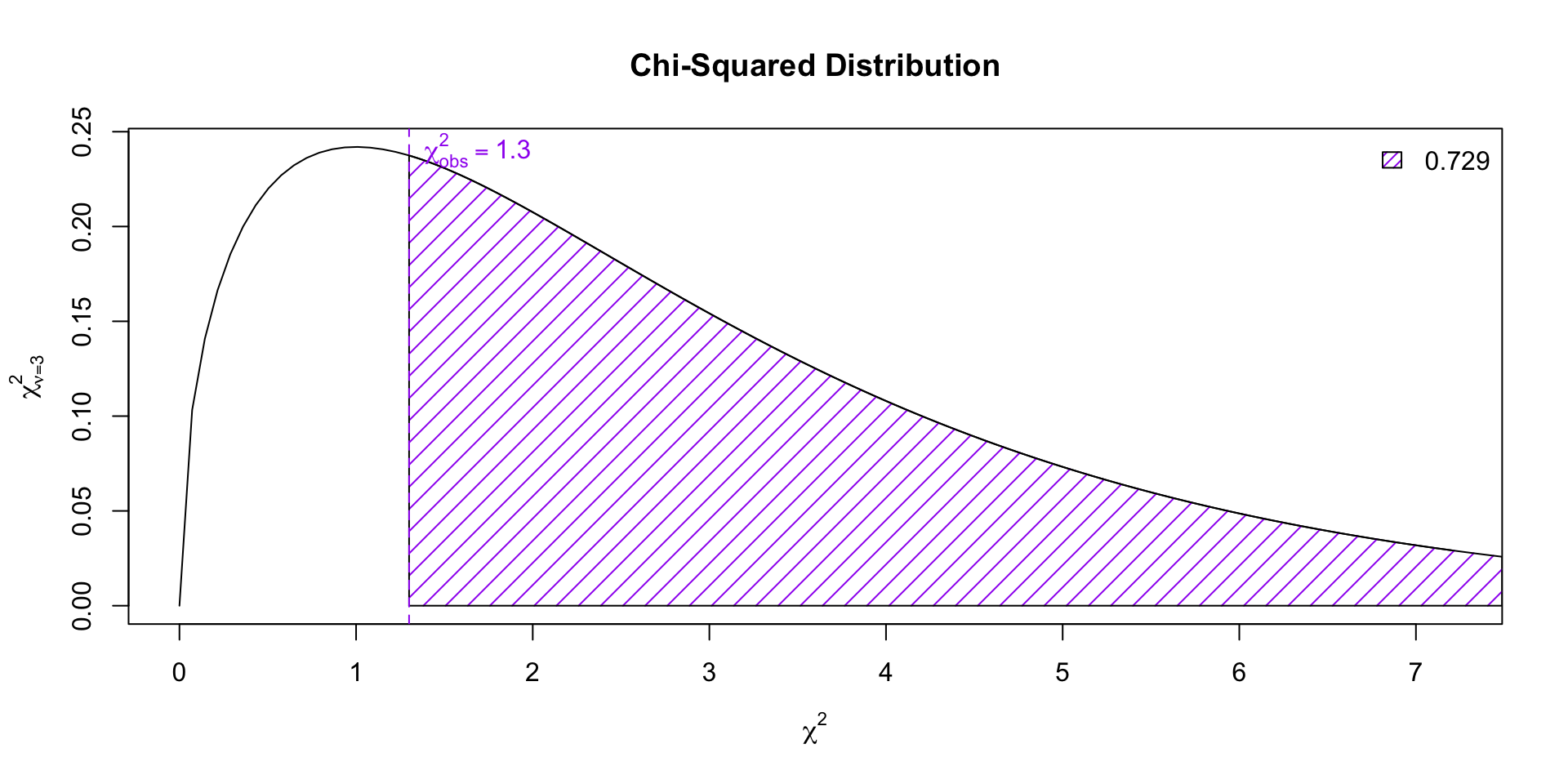
Conclusion

Since the \(p\)-value (0.729) is larger than \(\alpha = 0.05\), we fail to reject the null hypothesis that the distribution of hockey players’ birth months follows a uniform distribution across all four quarters.

In R

As we have seen with other hypothesis tests, rather than computing these tedious formulas “by hand”, we rely on software like R perform these calculations for us.

chisq.test(x, y = NULL, p = rep(1/length(x), length(x)))

• x a numeric vector or matrix. x and y can also both be factors.
• y a numeric vector; ignored if x is a matrix. If x is a factor, y should be a factor of the same length.
• p a vector of probabilities the same length as x

Alternatively, you could specify a contingency table, …

Political Opinion in R

Returning to Exercise 2, we could perform the test in R using the following code:

demo

     [,1] [,2] [,3]
[1,]  138   83   64
[2,]   64   67   84

chisq.test(demo)

    Pearson's Chi-squared test

data:  demo
X-squared = 22.152, df = 2, p-value = 1.548e-05

NHL in R

Returning to Exercise 3, we could perform the test in R using the following code

hockey_tab

bins
Jan-Mar Apr-Jun Jul-Sep Oct-Dec 
     24      20      19      17 

chisq.test(hockey_tab)

    Chi-squared test for given probabilities

data:  hockey_tab
X-squared = 1.3, df = 3, p-value = 0.7291

Example

Example: Type 2 Diabetes

The following contingency table summarizes the results of an experiment evaluating three treatments for Type 2 Diabetes in patients aged 10-17 who were being treated with metformin. The three treatments considered were continued treatment with metformin (met), treatment with metformin combined with rosiglitazone (rosi), or a lifestyle intervention program (lifestyle). Each patient had a primary outcome, which was either lacked glycemic control (failure) or did not lack that control (success). Perform the appropriate hypotheses test.

library(openintro)
library(tidyverse)
data(diabetes2)

Data

diabetes2

Contingency Table

table(diabetes2)

           outcome
treatment   failure success
  lifestyle     109     125
  met           120     112
  rosi           90     143

Hypothesis

\(H_0\): There is no difference in the effectiveness of the three treatments.

\(H_A\): There is some difference in effectiveness between the three treatments, e.g. perhaps the rosi treatment performed better than lifestyle.

R code

chisq.test(diabetes2$treatment, diabetes2$outcome)

    Pearson's Chi-squared test

data:  diabetes2$treatment and diabetes2$outcome
X-squared = 8.1645, df = 2, p-value = 0.01687

Since the \(p\)-value is less than \(\alpha = 0.05\) we reject the null hypothesis in favour of the alternative. That is to say, there is sufficient evidence to suggest that there is some difference in effectiveness between the three treatments.

Comment

• A two-proportion Z-test and a chi-squared test of independence are mathematically equivalent for 2×2 tables if the Z-test is two-sided

• Note: a one-sided Z-test has no direct chi-squared equivalent.

• Their test statistics are related: \(Z^2 = \chi^2\)

Exercise Revisited

Online Learning Resources

Are college students more likely to use online learning resources than high school students?

• Sample Data:
  • College students: 120 out of 200 use online resources (\(\hat{p}_1 = 0.60\)).
  • High school students: 90 out of 200 use online resources (\(\hat{p}_2 = 0.45\)).

Is there a difference in the likelihood of using online learning resources between college and high school students?

Code Comparison

# Two-proportion Z-test in R (built-in function)
prop.test(c(120, 90), c(200, 200), correct = FALSE)

...

data:  c(x1, x2) out of c(n1, n2)
X-squared = 9.0226, df = 1, p-value = 0.002667
alternative hypothesis: two.sided
95 percent confidence interval:
 0.05323453 0.24676547
sample estimates:
prop 1 prop 2 
  0.60   0.45 
...

# Chi-squared test (without continuity correction)
chisq.test(tab, correct = FALSE)

...

data:  tab
X-squared = 9.0226, df = 1, p-value = 0.002667
...

tab

           Used NotUsed
College     120      80
HighSchool   90     110

🎉 That’s a Wrap! 🎓

Thanks for a great term!

• 🌱 Keep practicing: Stats is a skill — the more you use it, the sharper it gets.
  
• 💬 Ask questions: Curiosity drives understanding.
  
• 📈 Think critically: Numbers are powerful — but context is everything.
  
• 💛 Be kind (especially to yourself): Learning takes time and effort. You did the work.
• 📝 Share your feedback: Please take a few minutes to complete the Student Experience of Instruction (SEI) survey

your feedback helps improve the course for future students.

and also supports my tenure and promotion process. 🙏