ANOVA

STAT 205: Introduction to Mathematical Statistics

Dr. Irene Vrbik

University of British Columbia Okanagan

Introduction

• At this point, we know how to perform inference for the difference of population means from two samples.

• To determine if the means from more than two populations are equal we use Analysis of Variance or ANOVA.

• ANOVA¹ can be considered an extension the (pooled) two-sample \(t\) procedure to more than two groups. However, it involves a test statistic falling a new distribution …

(independent and paired)

1. one-way ANOVA

Outline

In this lecture we will be covering

• Total Sum of Squares

• Mean Squares

• Test Statistic

• F-distribution

• Example: ANOVA Table

While we will be going through some of the “under-the-hood” calculations, I will not require that you do these “by-hand” as I did for the previous tests.

Review of Pooled t-test

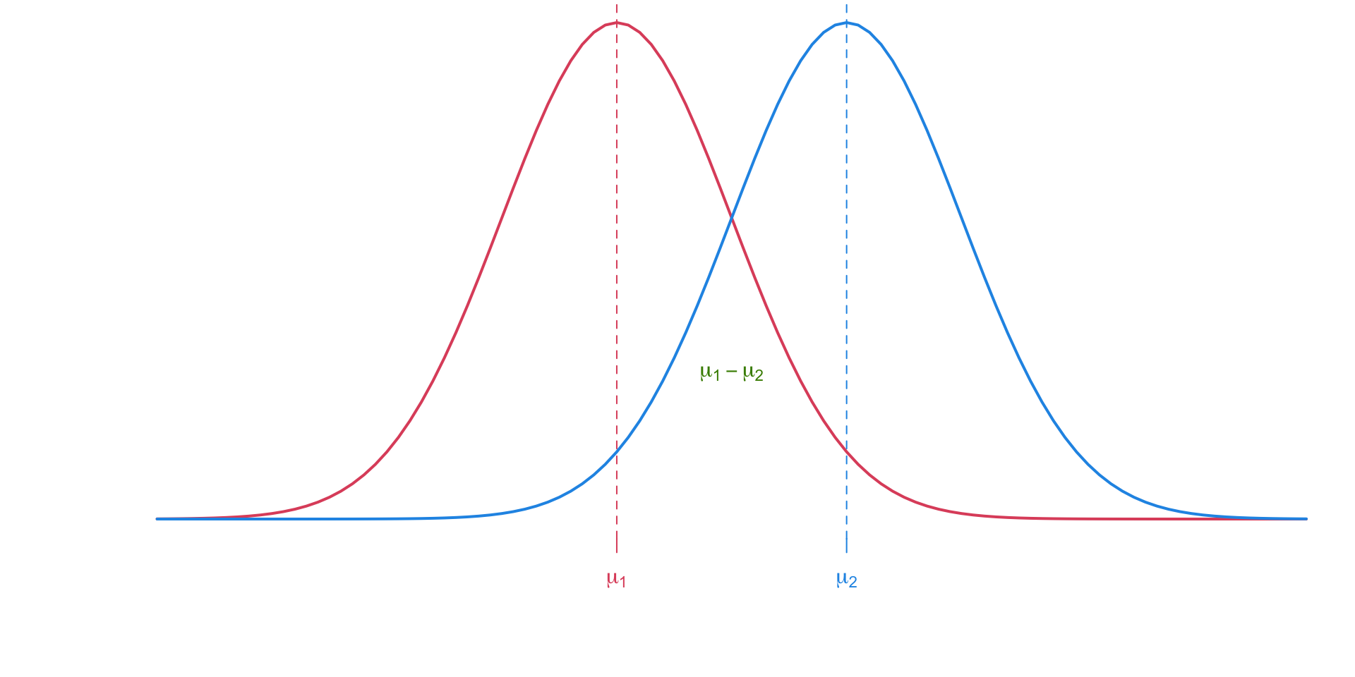
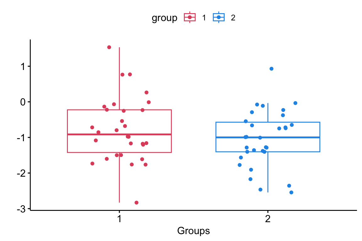
The pooled \(t\)-test assumes equal variance amoung two independent populations. Inference is done on the difference between the two population means \(\mu_1 - \mu_2\).

Pooled Null Hypothesis

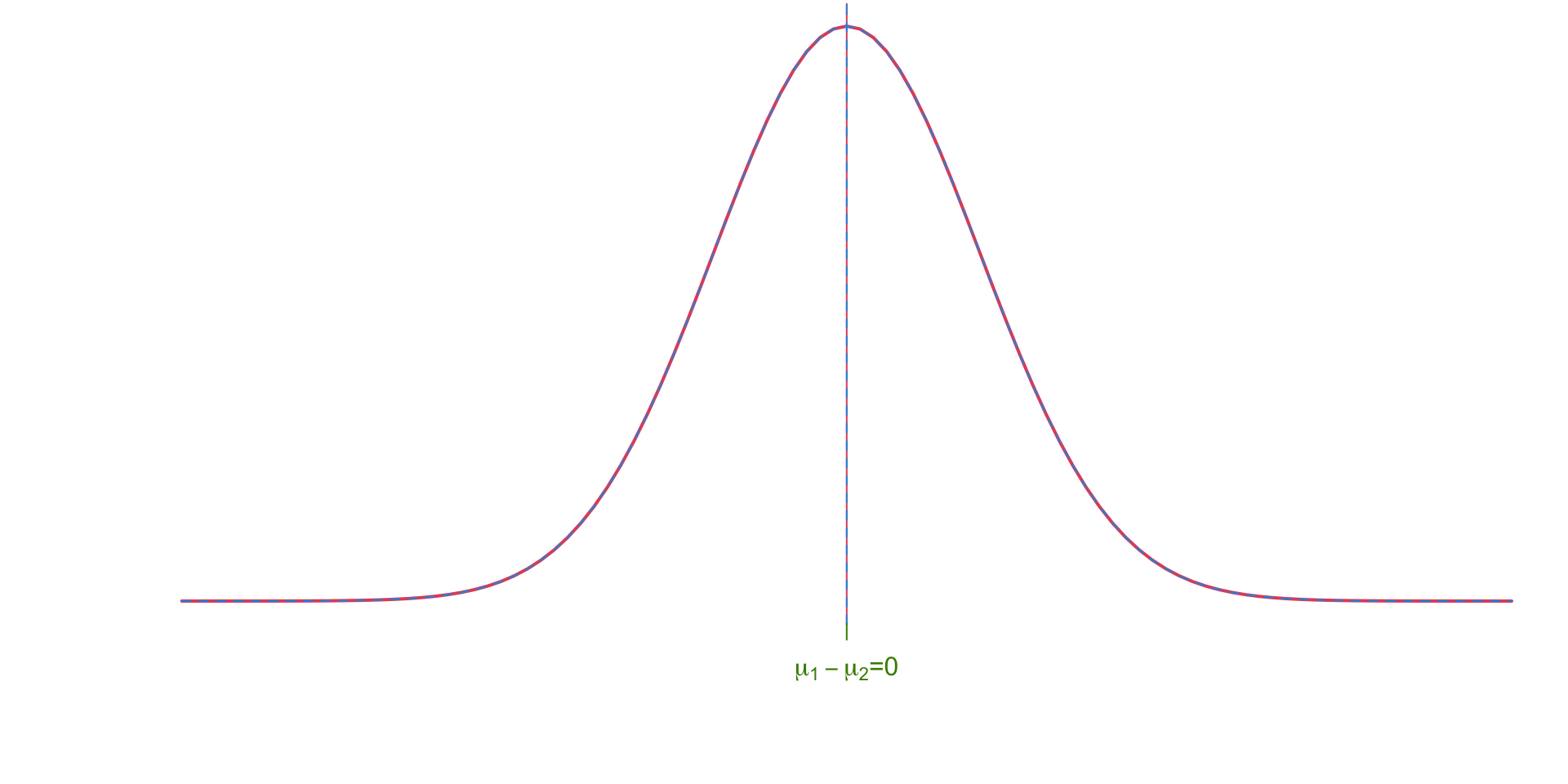
The null hypothesis assumes that there is no difference between the means of the two groups (i.e. \(\mu_1 - \mu_2 = 0)\).

Sample data

This sample data is consistent with null hypothesis; it produces a non-significant \(p\)-value = 0.2233208

This sample data provides sufficient evidence against the null hypothesis; it produces a significant \(p\)-value = 1.860976e-15

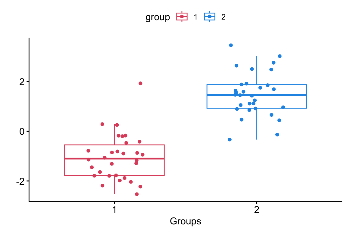
Comparing more than 2 groups

Now we seek to determine whether there are any statistically significant differences between the means of three or more independent groups.

ANOVA null hypothesis

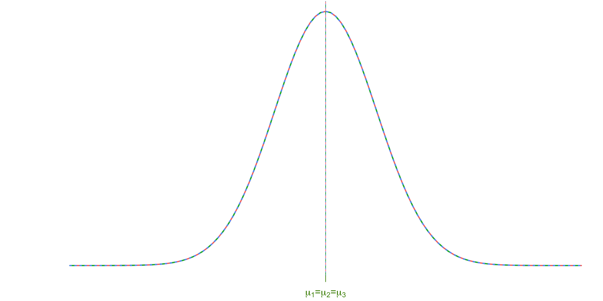
As with the pooled \(t\)-test, our null hypothesis will assume that all group means are equal. The ANOVA test will also require the equal population variance assumption.

Assumptions

In words and symbols, the assumptions of this so-call one-way ANOVA is similar to the pooled \(t\)-test:

1. The observations are independent simple random samples from the populations
2. The populations are normally distributed
3. The population variances are equal \[\sigma_1^2 = \sigma_2^2 = \dots = \sigma_k^2\]

The plausibility of independence of the samples (and of the individual observations within the samples) stems from a study’s design. At the end of this section we discuss methods for checking the plausibility of the normality and equal variance assumptions.

we sometimes same \(\sigma_1^2 = \sigma_2^2 = \dots = \sigma_k^2\) is equal to some common variance \(\sigma^2\).

Comment about assumptions

Non-extreme departures from the normality assumes are not that serious since the sampling distribution of the test statistic is fairly robust, especially as sample size increases sample sizes for all groups are equal.

If you conduct an ANOVA test, you should always try to keep the same sample sizes for each group; this is known as balanced study design.

A general rule of thumb for equal variances is to compare the smallest and largest sample standard deviations. This is much like the rule of thumb for equal variances for the test for independent means. If the ratio of these two sample standard deviations falls within 0.5 to 2, then it may be that the assumption is not violated.

Unequal sample sizes will be considered in Section 11.3.

Preamble

• The name ANOVA: Analysis of Variance is a bit misleading.

• Unlike it’s name suggests, ANOVA is a statistical methods used to investigate differences among the means.

• The test involves separating observed variance data into different components and assess whether the observed differences in the sample means are larger than would be expected due to random variation alone.

Example

Let’s examine the rationale behind ANOVA using the following example …

Tar content

Exercise 1 We want to see whether the tar contents (in milligrams) for three different brands of cigarettes are different. Two different labs took samples, Lab Precise and Lab Sloppy.

This question was adapted from Lesson 10 of Penn State STAT 500

Hypotheses

• The null hypothesis in ANOVA asserts that there is no significant difference among the means of the groups being compared, i.e.:

  \[H_0: \mu_1 = \mu_2 = \mu_3 = \ldots = \mu_k\]

  where \(\mu_1, \mu_2, \mu_3, \ldots, \mu_k\) are the population means of the \(k\) groups being compared.

• The alternative hypothesis in ANOVA suggests that at least one of the group means is significantly different from the others, i.e.:

  \[H_A: \text{ At least one } \mu_i \text{ is different from the others, }\]

  where \(i = 1, 2, 3, ..., k\).

This means that at least one of the pairs is not equal.

Data

library(tidyverse)
# Create the data
lab_precise <- data.frame(
  Sample = 1:6,
  Brand_A = c(10.21, 10.25, 10.24, 9.80, 9.77, 9.73),
  Brand_B = c(11.32, 11.20, 11.40, 10.50, 10.68, 10.90),
  Brand_C = c(11.60, 11.90, 11.80, 12.30, 12.20, 12.20)
)

lab_sloppy <- data.frame(
  Sample = 1:6,
  Brand_A = c(9.03, 10.26, 11.60, 11.40, 8.01, 9.70),
  Brand_B = c(9.56, 13.40, 10.68, 11.32, 10.68, 10.36),
  Brand_C = c(10.45, 9.64, 9.59, 13.40, 14.50, 14.42)
)

# Calculate the mean of Brand_C in both datasets
mean_brand_c_precise <- mean(lab_precise$Brand_C)
mean_brand_c_sloppy <- mean(lab_sloppy$Brand_C)

# Calculate the adjustment needed for Brand_C in both datasets
adjustment_precise <- 11.5 - mean_brand_c_precise
adjustment_sloppy <- 11.5 - mean_brand_c_sloppy

# Adjust Brand_C values in lab_precise
lab_precise$Brand_C <- lab_precise$Brand_C + adjustment_precise

# Adjust Brand_C values in lab_sloppy
lab_sloppy$Brand_C <- lab_sloppy$Brand_C + adjustment_sloppy

precise_stats <- lab_precise %>%
  select(-Sample) %>%
  summarise_all(mean)

sloppy_stats <- lab_sloppy %>%
  select(-Sample) %>%
  summarise_all(mean)

overall_mean = mean(unlist(lab_precise[,-1]))

lab_sloppy[,-1]

\[\begin{align} \bar x_A &= 10 & \bar x_B &= 11 & \bar x_C &= 11.5 \end{align}\]

lab_precise[,-1]

\[\begin{align} \bar y_A &= 10 & \bar y_B &= 11 & \bar y_C &= 11.5 \end{align}\]

Notice how the summary statistics are identical, but the individual values are clearly not.

Note that the overall mean tar content for across all sampled cigarettes in each lab are also identical \(\bar x = 10.83\)

Normality Check for Lab Sloppy

par(mfrow=c(1,3))
library(car)
out <- qqPlot(lab_sloppy$Brand_A, xlab = "", main = "Lab Sloppy Brand A")
out <- qqPlot(lab_sloppy$Brand_B, xlab = "", main = "Lab Sloppy Brand B")
out <- qqPlot(lab_sloppy$Brand_C, xlab = "", main = "Lab Sloppy Brand C")

Figure 1: To check our normality assumption we could do a qq-norm plot. Note that we will have to do this for each group in Lab Sloppy

one potential outlier to look out for

Normality Check for Lab Precise

par(mfrow=c(1,3))
library(car)
out <- qqPlot(lab_precise$Brand_A, xlab = "", main = "Lab Precise Brand A")
out <- qqPlot(lab_precise$Brand_B, xlab = "", main = "Lab Precise Brand B")
out <- qqPlot(lab_precise$Brand_C, xlab = "", main = "Lab Precise Brand C")

Figure 2: To check our normality assumption we could do a qq-norm plot. Note that we will have to do this for each group in Lab Precise

Normality Check

We could have checked normality using Shapiro Wilks.

shapiro.test(residuals(anova_sloppy))

    Shapiro-Wilk normality test

data:  residuals(anova_sloppy)
W = 0.93497, p-value = 0.2372

shapiro.test(residuals(anova_precise))

    Shapiro-Wilk normality test

data:  residuals(anova_precise)
W = 0.90362, p-value = 0.06646

Warning

For large samples, this test often gives small p-values even for minor deviations from normality. For small samples, this test is not very powerful.

✏️ Therefore, use visual aids as your main diagnostics, and use the Shapiro-Wilk test to supplement.

anova_sloppy and anova_precise will be defined later.

Homogeneity

The equal variance assumption can be checked using:

• Graphical Methods ✅ If the spreads (IQRs) of side-by-side boxplots look similar across groups

• Rule of Thumb ✅ Largest SD \(\leq\) 2 \(\times\) Smallest SD

• Statistical Tests¹

  • Levene’s Test (most common)
  • Bartlett’s Test (only use if confident the data are normal)

equal variance assumption (also called homogeneity of variances)

The assumption is supported when… 1. 2.

However, Lavenes test is flawed in two ways and should be avoided.

a) oversensitive with large samples: Negligible differences will cause the test to reject \(H_0\): data is normal

• i.e. likely to make a type I error.

b) lacks power with smaller samples, more likely to falsely fail to reject \(H_0\).

• i.e. more likely to commit a type II error.

1. Like Shapiro Wilks, these tests are flawed for small/large \(n\)

Hypotheses

While the hypotheses can by written in symbols using: \[\begin{align} H_0:& \mu_1 = \mu_2 = \dots = \mu_k & H_A:& \mu_i \neq \mu_j \text{ for some $i\neq j$} \end{align}\] they are often expressed in plain language as:

• \(H_0\): All group means are equal
• \(H_A\): not all means are equal
• OR \(H_A\): at least one mean is different (more common)

Boxplots Sloppy Labs

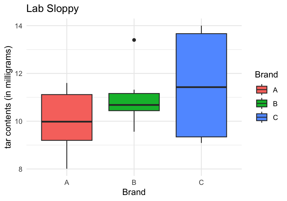
Would you guess that the difference in means for the “Sloppy” labs is significantly different?

iClicker

1. Yes
2. No
3. I have no idea

Boxplots Precise Labs

How about for the Precise Lab? Would you guess the difference in means is statistically significant?

iClicker

1. Yes
2. No
3. I have no idea

Boxplots

This sample data is consistent with \(H_0: \mu_A = \mu_B = \mu_C\);
it produces a non-significant \(p\)-value = 0.345451

This sample data provides sufficient evidence against \(H_0: \mu_A = \mu_B = \mu_C\) in favour of the alternative; it produces a significant \(p\)-value = 1.301632e-06

remember the means are the same, the sample means from the two labs turned out to be the same and thus the differences in the sample means from the two labs are zero.

There is substantial amount of overlap among observations on the first Sloppy lab , but not in second Precise lab.

These graphs suggest that it’s insufficient to consider only how far apart the sample means are in assessing whether the population means are different; we must also account for the amount of variability within each of the I samples

The p-value is significant for Precise labs, this suggests that there is evidence to suggest that the tar content in these three brands of cigarettes is significantly different.

.

Comments

• The sample means from the two labs turned out to be the same, however, the data from Lab Precise produces a significant \(p\)-value whereas Lab Sloppy does not.
• These graphs suggest that it’s insufficient to consider only how far apart the sample means are in assessing whether the population means are different; we must also account for the amount of variability within each of the I samples

• The difference between these two samples is apparent in the variability within groups, i.e. the boxplots from Lab Sloppy are much wider than Lab Precise.

• Since the between-sample-variation from Lab Sloppy is large compared to the within-sample-variation for data from Lab Precise, we will be more inclined to conclude that the three population means are different using the data from Lab Precise.

• In order to do an ANOVA test, we will be comparing the between-sample-variation to the within-sample-variation.

Notation

Group	Data	Mean
1	\(y_{11}, y_{12}, \dots, y_{1n_1}\)	\(\bar y_{1\cdot}\)
2	\(y_{21}, y_{22}, \dots, y_{2n_2}\)	\(\bar y_{2\cdot}\)
\(\vdots\)	\(\vdots\)	\(\vdots\)
\(k\)	\(y_{k1}, y_{k2}, \dots, y_{kn_k}\)	\(\bar y_{3\cdot}\)

• \(k\) total number of groups
• \(y_{ij}\) the \(j\)th observation from the \(i\)th group
• \(n_i\) the sample size from the population
• \(n = \sum_{i=1}^k\) the total sample size

• \(\bar y_{i\cdot}\) the sample mean from the \(i\)th population, i.e. \(y_{i\cdot} = \frac{1}{n_i} \sum_{j=1}^{n_i} y_{ij}\), for \(i = 1, \dots, k\)
• \(\bar y_{\cdot\cdot}\) the overall mean, i.e. \(\bar y_{\cdot\cdot} = \frac{1}{n}\sum_{i = 1}^k \sum_{j=1}^{n_i} y_{ij}\)
• overall sample variance \(s^2 = \frac{1}{n - 1}\sum_{i=1}^{k}\sum_{j=1}^{n_i} (y_{ij} - \bar y_{\cdot\cdot})^2\)
• group sample variance \(s_i^2 = \frac{1}{n_i - 1}\sum_{j=1}^{n_i} (y_{ij} - \bar y_{i\cdot})^2\)

it is customary to use a single letter with two subscripts. The first subscript identifies the sample number, corresponding to the population or treatment being sampled, and the second subscript denotes the position of the observation within that sample. Let

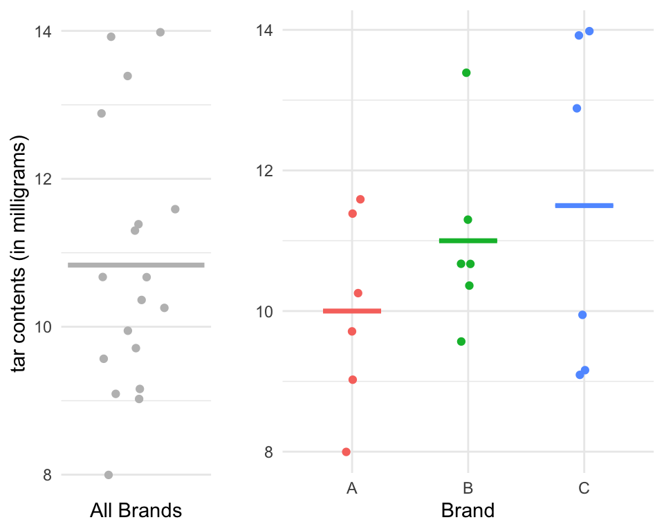
Lab Sloppy

Left: Dot plot showing the tar levels of the sample from Lab Sloppy; the overall mean \(y_{\cdot\cdot} = 10.83\) is depicted as a horizontal gray line. Right: a plot of the tar levels for each brand of cigarettes, grouped and coloured by brand. The group means \(y_{1\cdot}\), \(y_{2\cdot}\), and \(y_{3\cdot}\), are indicated using the pink, green, and blue horizontal line, respectively.

Lab Precise

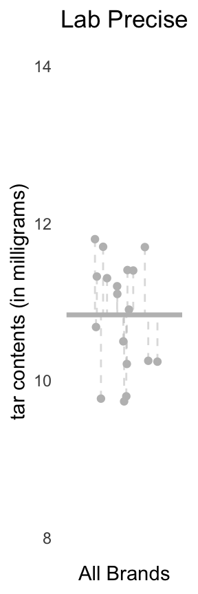
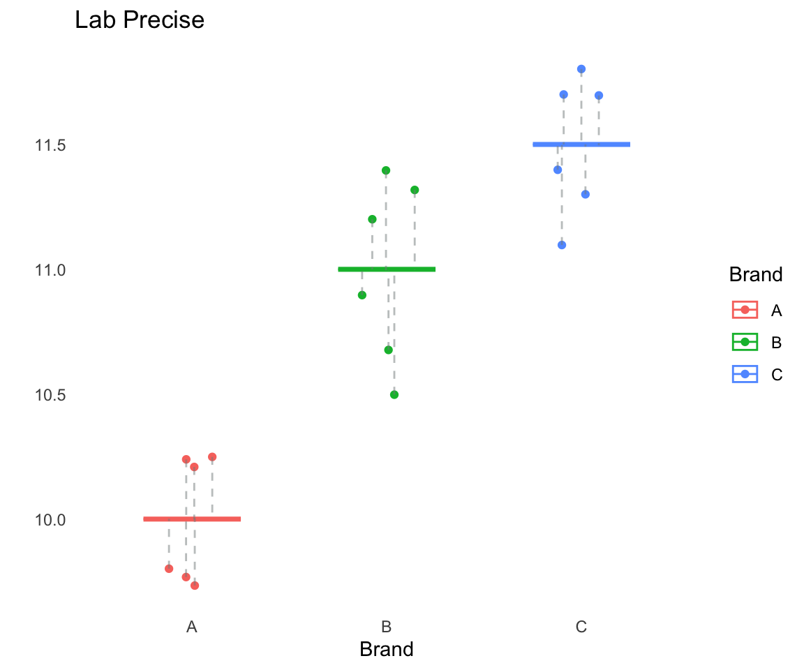
Left: Dot plot showing the tar levels of the sample from Lab Precise; the overall mean \(y_{\cdot\cdot} = 10.83\) is depicted as a horizontal gray line. Right: a plot of the tar levels for each brand of cigarettes, grouped and coloured by brand. The group means \(y_{1\cdot}\), \(y_{2\cdot}\), and \(y_{3\cdot}\), are indicated using the pink, green, and blue horizontal line, respectively.

Total Sum of Squares

The total sum of squares¹ is given by: \[\begin{equation} TSS = \sum_{i,j} (y_{ij} - y_{\cdot \cdot})^2 \end{equation}\]

For Lab Sloppy: \[TSS = 52.9756\]

For Lab Precise: \[TSS = 8.3748\]

Recall that we want to examine the between group variation and the within group variation. We can find an estimate of the variations with the following:

1. this is the numerator of the sample variance of all the sample data

Decomposition of TSS

It can be shown that the \(TSS\) can be decomposed into:

• SSW: the within sum of squares, also known as the Sum of Squares for Error and the
• SSB: the between sum of squares, also known as the Sum of Squares for Treatment

\[\begin{equation} TSS = SSW + SSB \end{equation}\]

• SST is a measure of the total variation in the data—the sum of all squared deviations about the grand mean. it can be partitioned into two pieces.

• So i want to figure out how much of this total ss (TSS) is due the the variance within vs between the two groups.

• SSB is the amount of variation (between samples) that can be explained by possible differences in the \(\mu_i\)’s: when the \(\mu_i\)’s differ substantially, the individual sample means should be further from the grand mean than when the \(\mu_i\)’s are identical or close to one another.

• SSW measures variation that would be present (within samples) even if \(H_0\) were true; thus, SSW the part of total variation that is unexplained by the truth or falsity of \(H_0\). If explained variation is large relative to unexplained variation, then H0 should be rejected in favor of Ha.

Note

Some texts use SSE instead of SSW and SST/SSTr instead of SSB (which gets easily confused with total sum of squares)

Definition of SSW and SSB

The SSW is a measure of variation within groups. The formula combines the variability within each sample separately \[ SSW = \sum_{i = 1}^ k \sum_{j = 1}^{n_i} (Y_{ij} - \bar Y_{i\cdot})^2 = \sum_{i,j} (Y_{ij} - \bar Y_{i\cdot})^2 \] The SSB is a measure of the variation between groups. The formula assesses variation in the means from the different samples: \[ SSB = \sum_{i = 1}^{k} \sum_{j = 1}^{n_i} (\bar Y_{i\cdot} - \bar Y_{\cdot\cdot})^2 = \sum_{i = 1}^{k} n_i (\bar Y_{i\cdot} - \bar Y_{\cdot\cdot})^2 \]

SSW entails assessing variability within each sample separately (via the sample variance) and then combining these assessments. \[\begin{align} SSW &= \sum_{i = 1}^ k \sum_{j = 1}^{n_i} (Y_{ij} - \bar Y_{i\cdot})^2 \\ &= \sum_{i = 1}^ k (n_i - 1) \sum_{j = 1}^{n_i- 1} \frac{(Y_{ij} - \bar Y_{i\cdot})^2}{n_i} \\ &= \sum_{i = 1}^ k (n_i - 1) S_i^2 \\ \end{align}\]

Lab Sloppy: Within Sum of Squares

\[\begin{align} SSW &= \sum_{i,j} (y_{ij}- \bar y_{i\cdot})^2\\ &= 45.9756 \end{align}\]

where

• \(\bar y_{1\cdot} = 10\)
• \(\bar y_{2\cdot} = 11\)
• \(\bar y_{3\cdot} = 11.5\)

within-samples variation (assessing variation separately within each sample and then combining).

so rather than taking the squared difference between points and the grand mean, we are taking the squared differences, between teh points and their group mean

• SSW measures variation that would be present (within samples) even if \(H_0\) were true

Lab Precise: Within Sum of Squares

\[\begin{align} SSW &= \sum_{i,j} (y_{ij}- \bar y_{i\cdot})^2\\ &= 1.3748 \end{align}\]

where

• \(\bar y_{1\cdot} = 10\)
• \(\bar y_{2\cdot} = 11\)
• \(\bar y_{3\cdot} = 11.5\)

within-samples variation (assessing variation separately within each sample and then combining).

The SSW is much large for lab sloppy (45.9756) since it exhibits much greater within-samples variation than does the lab precise

Lab Sloppy: Between Sum of Squares

between-samples variation (i.e., the disparity between the \(k\) sample means)

• SSB represents the variation between samples; when the population means differ significantly, the sample means are expected to deviate farther from the grand mean compared to scenarios where the population means are similar.

• Notice how the SSW is making up most of the variation here and SSW is much bigger than SSB

• there is more variation between groups than there is within groups

\[\begin{align} SSB &= \sum_{i=1}^k n_i(\bar y_{i\cdot}- \bar y_{\cdot\cdot})^2\\ &= 6(10 - 10.83)^2 \\ &+6(11- 10.83)^2 \\ &+6(11.5- 10.83)^2 \\ &= 7 \end{align}\]

\[\begin{align} TSS&= 52.9756\\ &= SSB + SSW\\ &= 7 + 45.9756\\ \end{align}\]

Lab Precise: Between Sum of Squares

The between sum of squares, also known as the Sum of Squares for Treatment is given by

between-samples variation (i.e., the disparity between the \(k\) sample means)

\[\begin{align} SSB &= \sum_{i=1}^k n_i(\bar y_{i\cdot}- \bar y_{\cdot\cdot})^2\\ &= 6(10 - 10.83)^2 \\ &+6(11- 10.83)^2 \\ &+6(11.5- 10.83)^2 \\ &= 7 \end{align}\]

\[\begin{align} TSS&= 8.3748\\ &= SSB + SSW\\ &= 7 + 1.3748\\ \end{align}\]

SSB is the same for lab precise as lab sloppy since the group means are the same

However the SSW is much smaller than SSB. In other words, there is more variation between groups than there is within groups

Comments

• SSB captures the variation between the sample means that can be “explained” by differences in \(\mu_i\)s; when the population means differ significantly SSB will be large¹

• SSW represents the “unexplained” variation, as it captures the variation within each sample that remains even if the null hypothesis is true.

• If the explained variation, SSB, is significantly larger than the unexplained variation SSW, we should reject \(H_0\).

• SST quantifies the overall variability in the data, encompassing all squared deviations from the grand mean.

• on the flip side, SSB will be smaller in scenarios where the population means are similar.

1. on the slip side, when the population means are similar, SSB should be small

Total Variance

Recall that we want to examine the between group variation and the within group variation. You may notice that the TSS given by: \[\begin{equation} TSS = \sum_{i,j} (y_{ij} - \bar y_{\cdot \cdot})^2 \end{equation}\] is the numerator of the sample variance of all the sample data, i.e.  \[\begin{equation} \text{Overall Sample Variance} = \frac{TSS}{df_t} \end{equation}\] where \(df_t = n - 1\) is the total Degrees of Freedom. When we divide the total SS by it’s df we get the Mean Squares Total (MST).

the sum of squares (SS) represents the total variability in the data. To make these measures comparable across different sources of variation, such as between groups and within groups, they are divided by their respective degrees of freedom.

Degrees of freedom

• \(SSB\) and \(SSW\) are on difference scales so we can not (yet) directly compare them.
• To address this, we calculate analogous Mean Squares metrics, which are obtained by dividing the sum of squares by its corresponding degrees of freedom, \(df\)¹
• The resulting \(MSB\) and \(MSW\) are comparable, allowing us to assess the relative contribution of between-group and within-group variability to the total variability in the data.

units (we expect more variability in individual points than with the variability in means)

• SSB measures the variability between group means, whereas
• SSW measures the variability within each group.

Comparing them directly without considering this difference in scale can be misleading.

SSB and SSW have different degrees of freedom

• SSB has degrees of freedom equal to the number of groups minus one (\(k-1\))
• SSW has degrees of freedom equal to the total sample size minus the number of groups (\(n-k\)). This difference in degrees of freedom affects the interpretation of the sum of squares.

1. df represent the number of independent pieces of information available for estimating a parameter or testing a hypothesis; see these videos for more insight [1] [2].

Formula Summary

Sum of Squares

The Between group Sum of Squares: \[\begin{equation} SSB = \sum_{i=1}^k n_i(\bar y_{i\cdot}- \bar y_{\cdot\cdot})^2 \end{equation}\] The Within Group Sum of Squares: \[\begin{equation} SSW = \sum_{i = 1}^ k \sum_{j = 1}^{n_i} (Y_{ij} - \bar Y_{i\cdot})^2 := \sum_{i,j} (Y_{ij} - \bar Y_{i\cdot})^2 \end{equation}\] Total Sum of Squares (TSS): \[\begin{align} TSS &= \sum_{i,j} (y_{ij} - y_{\cdot \cdot})^2 = SSB + SSW \end{align}\]

Mean Squares

The mean square for between groups \[\begin{equation} MSB = \dfrac{SSB}{k - 1} = \dfrac{SSB}{df_B} \end{equation}\] The mean square for error is \[\begin{equation} MSW = \dfrac{SSW}{n -k} = \dfrac{SSW}{df_W} \end{equation}\] The mean square total is \[\begin{equation} MST = \dfrac{TSS}{n - 1} = \dfrac{TSS}{df_T} \end{equation}\]

• The word “mean” is being used in the sense of average;

• a “mean square” is a sum of squares divided by its associated degrees of freedom.

• Thus SSB assesses variation in the means from the different samples, whereas SSW entails assessing variability within each sample separately (via the sample variance) and then combining these assessment

\(SSB\)/\(MSB\) more often called \(SST\)/\(MST\) or \(SSTr\)/\(MSTr\) (for treatment), \(SSW\)/\(MSW\) is sometimes called \(SSE\)/\(MSE\) (for error)

Test Statistic

\[\begin{align} F &= \dfrac{\text{between group variance}}{\text{within group variance}}= \dfrac{{MSB}}{MSW} \end{align}\]

• This test statistic follows a so-called F-distribution.
• Under \(H_0\), this ratio should be close to 1¹
• On the contrary, large values of large F-values indicate differences between groups.

The test statistic for One-Way ANOVA is given by:

If \(H_0\) is true, both the numerator (between-groups variability) and the denominator (within-groups variability) are estimates of \(\sigma^2\) .

Consequently, the F-ratio should be close to 1 when there are no true differences between the group means.

1 implies Sampling variability alone explains the differences between group means.

\(>1\implies\) that the between-groups variability is much larger than the within-groups variability and likely differences between the group means

1. under \(H_0\) the numerator the denominator should provide similar estimates of \(\sigma^2\). See 11.1 of Devore, Berk, and Carlton (2021) for details

F-distribution

An \(F\)-distribution has two parameters:

• \(\nu_1\) “numerator” df
• \(\nu_2\) “denominator” df

We denote the r.v. \(F_{\nu_1, \nu_2}\)

For one-way ANOVA:

• \(\nu_1 = df_B\) = Number of groups \(= k - 1\)
• \(\nu_2 = df_W\) = Total observations - Number of groups = \(n - k\)

numerators (measures variation between group means)

Example: Test Statistic

Back to Exercise 1, our test statistic (i.e. our \(F\)-ratio = \({MSB}/{MSW}\)) follows an \(F_{2, 15}\):

Large F-score

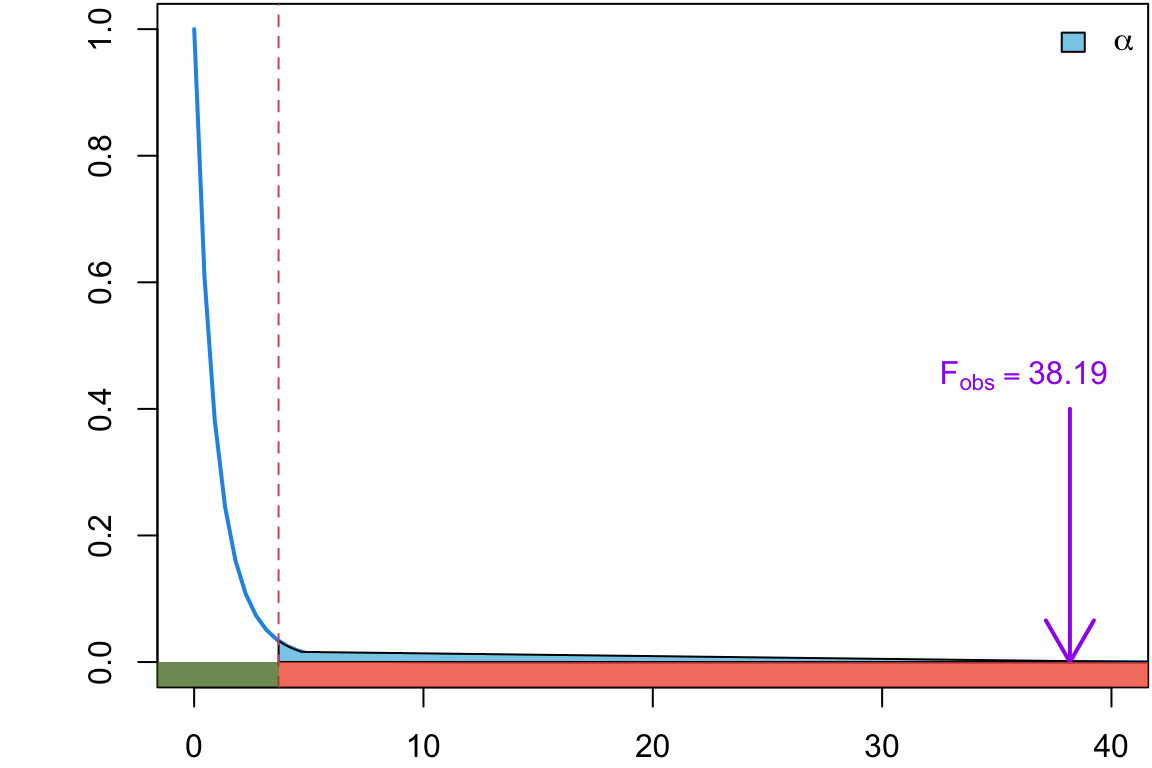
We mentioned that we will reject the null when \(F\) is too big. How big it too big?

Critical Value

How big it too big? \(F_{crit}\) = 3.68

qf(0.05, df1 = k - 1, df2 = n - k, lower.tail = FALSE) # = F_crit
qf(0.95, df1 = k - 1, df2 = n - k) # equivalent to above

this rejection region is always in the upper tail

ANOVA is a one-sided test — we only reject the null when \(F\) is too big, i.e., when between-group variability is much larger than within-group variability.

(we don’t have any two-sided or lower tail alternatives)

Number Summary

Lab Sloppy:
SSB =7, SSW =45.9756,
MSB = 3.5, MSW =3.065 and \[F_{obs} = 1.14\]

Lab Precise:
SSB =7, SSW =1.3748,
MSB = 3.5, MSW =0.092 and \[F_{obs} = 38.19\]

Decision Summary

Since \(F_{obs}\) falls outside of the rejection region we fail to reject the null hypothesis

Since \(F_{obs}\) falls well inside of the rejection region we reject the null hypothesis

p-values

More commonly we will base our decision on a \(p\)-value.

\[ p\text{-value} = \Pr(F_{df_B, df_W} > F_{obs}) \]

Lab Sloppy

\[ \begin{align} &= \Pr(F_{2, 15} > 1.14)\\ &= 0.345451 \end{align} \]

Lab Precise

\[ \begin{align} &= \Pr(F_{2, 15} > 38.19)\\ &= 1.3016316\times 10^{-6} \end{align} \]

We can use pf() in R, but we usually get p-values directly from the aov() output.

pval_sloppy <- pf(1.14, df1 = 2, df2 = 15, lower.tail = FALSE)
pval_precise <- pf(38.19, df1 = 2, df2 = 15, lower.tail = FALSE)

p-value plots

Since the \(p\)-value is greater than \(\alpha\) we fail to reject the null hypothesis

Since the \(p\)-value is smaller than \(\alpha\) we reject the null hypothesis

Finding F-crit/p-values

• While \(F\)-distribution tables exists, they are usually multiple pages long and cumbersome to read off of.

• For this course I will not bother with the \(F\)-tables, and will either provide the \(p\)-value for the ANOVA tests, use examples for which the decision is apparent.

• Hence, you have some intuition that a very large \(F\)-ratio (e.g. Lab Precise \(F_{obs}\) = 38.19) would produce a very small \(p\)-value, and values close to one (e.g. Lab Sloppy \(F_{obs}\) = 1.14) would yield a large \(p\)-value.

ANOVA table

ANOVA table

These calculations are done using software like R and typically stored in an ANOVA table with this structure.

Source	df	SS	MS	F	\(p\)-value
Between	\(k - 1\)	SSB	MSB	\(\frac{MSB}{MSW}\)	\(\Pr(F_{df_B, df_W} > F_{obs})\)
Within	\(n- k\)	SSW	MSW
Total	\(n-1\)	TSS

• \(df_T = df_B + df_W\) \(= (k - 1) + (n-k) = n - 1\)
• \(TSS = SSW + SSB\)
• \(MSB = SSB/df_b\), \(MSW = SSW/df_W\)

Example: ANOVA Table

Returning to our Exercise 1, the ANOVA table for Sloppy labs:

Source	df	SS	MS	F	\(p\)-value
Between	2	7	3.5	1.1419101	0.345451
Within	15	45.9756	3.06504
Total	17	52.9756

ANOVA table

Source	df	SS	MS	F	\(p\)-value
Between	\(k - 1\)	SSB	\(\dfrac{SSB}{k-1}\)	\(\dfrac{MSB}{MSW}\)	\(\Pr(F_{df_B, df_W} > F_{obs})\)
Within	\(n- k\)	SSW	\(\dfrac{SSW}{n-k}\)
Total	\(n-1\)	TSS

Data format

Very commonly, your data will appear in “wide” format where each column represents a different group (Brand) and the rows represent samples.

lab_sloppy

From wide to long

• In these situations, you would have transform your data to “long” format such that each observation occupies a single row, with the variable(s) represented in columns. l

• For our example, each sampled cigarette would appear in the rows and we would have a single column corresponding to Brand (this is a factor with levels: A, B, or C)

• We can achieve this in various ways, e.g. using reshape() , melt() or pivot_longer() functions to name a few.

long table

Note: lab_sloppy and lab_precise defined on Data slide

library(tidyverse)

# Reshape the data from wide to long format
sloppy_long <- pivot_longer(lab_sloppy, cols = starts_with("Brand"), 
                            names_to = "Brand", values_to = "Value")

# Modify the "Brand" column to only show the letters 'A', 'B', and 'C'
# i.e. change Brand_A, Brand_B, Brand_C to A, B, C
sloppy_long <- sloppy_long %>%
  mutate(Brand = substr(Brand, nchar(Brand), nchar(Brand)))

# same for Lab Precise:
precise_long <- pivot_longer(lab_precise, cols = starts_with("Brand"), 
                             names_to = "Brand", values_to = "Value") %>%
  mutate(Brand = substr(Brand, nchar(Brand), nchar(Brand)))

sloppy_long

precise_long

ANOVA in R

You can fit an analysis of variance model in R using aov()

aov(formula, data = NULL)

the first argument is the formula which has the following form:

response_variable ~ group_variable

• response_variable = variable whose variation you are interested in explaining or predicting based on the grouping variable.
• group_variable = the categorical variable that defines the groups or categories in your data. Each level of the grouping variable represents a different group/population
• ~ separates the left-hand side (response variable) from the right-hand side (predictors)

Sloppy ANOVA Table

Returning to our Exercise 1, the ANOVA table for Sloppy labs becomes:

Source	df	SS	MS	F	\(p\)-value
Between	2	7	3.5	1.1419101	0.345451
Within	15	45.9756	3.06504
Total	17	52.9756

And in R…

anova_sloppy <- aov(Value ~ Brand, data = sloppy_long)
summary(anova_sloppy)

            Df Sum Sq Mean Sq F value Pr(>F)
Brand        2   7.00   3.500   1.142  0.345
Residuals   15  45.98   3.065               

Precise ANOVA Table

Returning to our Exercise 1, the ANOVA table for Precise labs becomes:

Source	df	SS	MS	F	\(p\)-value
Between	2	7	3.5	38.1873727	1.3016316^{-6}
Within	15	1.3748	0.0916533
Total	17	8.3748

And in R…

anova_precise <- aov(Value ~ Brand, data = precise_long)
summary(anova_precise)

            Df Sum Sq Mean Sq F value  Pr(>F)    
Brand        2  7.000   3.500   38.19 1.3e-06 ***
Residuals   15  1.375   0.092                    
---
Signif. codes:  0 '***' 0.001 '**' 0.01 '*' 0.05 '.' 0.1 ' ' 1

Decision

• As usual, if the \(p\)-value is less than our predefined significance level \(\alpha\), we reject the null hypothesis.

• Reject \(H_0 \implies\) conclude that not all the means are equal: that is, at least one mean is different from the other means.

• Notice there is no indication on which mean or means are statistically different (is one or multiple brands were better/worse than another?).

• In Exercise 1, a follow up question might be which brands differ in average tar content.

Multiple Comparison

• To answer this follow-up question we conduct an analysis of all possible pairwise means.

• This involves a method called multiple comparisons. ¹

• For Exercise 1, with three brands of cigarettes, A, B, and C, we would compare the three possible pairwise comparisons:

  1. Brand A to Brand B \(H_0: \mu_A = \mu_B\)

  2. Brand A to Brand C \(H_0: \mu_A = \mu_C\)

  3. Brand B to Brand C \(H_0: \mu_B = \mu_C\)

1. One commonly used is Fisher’s least significant difference (LSD) test or pairwise \(t\)-tests with Bonferroni correction; see ?pairwise.t.test

Summary

• ANOVA is a formal hypothesis test for multiple means that compares the within variation and between variation.

• The one-way ANOVA showed statistically significant results for Lab Precise but not for Lab Sloppy.

• Lab Precise: the within variation was small compared to the between variation thus resulted in a large F-statistic (38.1873727) and thus a small p-value (1.301632e-06).

• Lab Sloppy: this ratio was small (1.1419101), resulting in a large p-value (0.345451).

References

Material from this lecture has been adapted from “Statistics Online: Courses, Resources, and Materials. (n.d.). Retrieved from https://online.stat.psu.edu/stat500/”

Devore, J. L., K. N. Berk, and M. A. Carlton. 2021. Modern Mathematical Statistics with Applications. Springer Texts in Statistics. Springer International Publishing. https://books.google.ca/books?id=ghcsEAAAQBAJ.

Nishishiba, M., M. Jones, and M. Kraner. 2013. Research Methods and Statistics for Public and Nonprofit Administrators: A Practical Guide. SAGE Publications. https://books.google.ca/books?id=-EIXBAAAQBAJ.