Bagging, Boosting, and Classification and Regression Trees (CART)

Author

Dr. Irene Vrbik

Published

December 1, 2024

Overview

In this lab, you’ll explore three powerful tree-based methods: Classification and Regression Trees (CART), bagging, and boosting. You’ll learn to implement these techniques in R using both classification and regression tasks, interpret the results, and compare model performances.

Learning Objectives

Train and evaluate CART models for classification and regression tasks.
Apply bagging (using random forests) to improve predictive performance.
Use boosting to enhance model accuracy.
Compare the performance of these methods.

For classification, use the iris dataset. For regression, use the Boston dataset from the MASS package.

Packages Required

We’ll use the rpart, randomForest, gbm, caret, and MASS packages¹. If you don’t have them installed, install them by running the following command²:

install.packages(c("rpart", "randomForest", "gbm", "caret", "MASS"))

Methods

CART

CART is a tree-based algorithm that recursively splits the data into subsets based on the feature that provides the best separation of the classes. The result is a tree structure where each internal node represents a decision on a feature, and each leaf node represents a class label. This method is intuitive and interpretable, making it a popular choice for classification tasks.

In lecture I used the tree package; an earlier implementation of decision trees, to show the intermediate steps of building and pruning a tree. Both rpart and tree are R packages used for creating decision trees, but rpart is more flexibile and has advanced features, e.g., more control over the tree-building process, automatic pruning, built-in cross validation (as opposed to using a separate step using cv.tree()). It has a nice vignette here: https://cran.r-project.org/web/packages/rpart/vignettes/longintro.pdf

The general usage of rpart:

rpart(formula, data, method, control)

Arguments:

formula: Specifies the model in the format response ~ predictors. For example, Species ~ . means predicting Species using all other variables in the dataset.
data: The dataset containing the variables mentioned in the formula.
method: Specifies the type of model. The common options are:
- "class" for classification (categorical response).
- "anova" for regression (continuous response).
control: (Optional) Allows control over the tree-building process with parameters such as the minimum number of observations in a node before splitting (minsplit) or the maximum depth of the tree (maxdepth).

Note that rpart performs the growing and the cross-validation pruning in one call.

Random Forests

The randomForest function (from the package fo the same name) in R is used to build a random forest model, which is an ensemble learning method for classification and regression tasks. The basic usage of the function is:

# For classification
rf_model_class <- randomForest(Species ~ ., data = iris, ntree = 500, mtry = 2, importance = TRUE)

# For regression
rf_model_reg <- randomForest(medv ~ ., data = Boston, ntree = 500, mtry = 6, importance = TRUE)

Important Parameters:

formula: A formula describing the model to be fitted (e.g., Species ~ . for classification).
data: The dataset used for training.
ntree: Number of trees in the forest. More trees generally improve performance, but the gain diminishes after a certain point. Common values range from 100 to 1000.
mtry: Number of variables randomly sampled at each split. Smaller values introduce more randomness, while larger values may reduce the diversity among trees.
importance: If set to TRUE, measures the importance of each feature for prediction, allowing for variable importance plots.

Outputs:

$predicted: The predicted values (class labels for classification, predicted values for regression).
$importance: Variable importance measures, showing how much each feature contributes to the predictive accuracy.
$ntree: The number of trees actually grown in the forest.
$mtry: The number of variables tried at each split.

Boosting using `gbm`

The gbm (Generalized Boosted Models) package in R is used for implementing gradient boosting for both regression and classification tasks. Gradient boosting is an ensemble learning technique that builds multiple decision trees in a sequential manner, where each tree tries to correct the errors made by the previous ones. This approach can produce highly accurate predictive models by combining the strengths of multiple weak learners (shallow trees).

General Usage:

# Train a gradient boosting model for regression
gbm_model <- gbm(
  formula = medv ~ .,        # The model formula
  data = train_boston,       # Training data
  distribution = "gaussian", # Loss function for regression (gaussian for squared error)
  n.trees = 100,             # Number of trees to build
  interaction.depth = 3,     # Maximum depth of each tree
  shrinkage = 0.01,          # Learning rate (step size reduction)
  n.minobsinnode = 10,       # Minimum number of observations in the terminal nodes
  cv.folds = 5               # Number of cross-validation folds for evaluation
)

Important Parameters:

formula: Specifies the response variable and the predictors.
data: The dataset used to train the model.
distribution: Specifies the type of loss function. Common options include "gaussian" for regression and "bernoulli" for binary classification.
n.trees: The number of boosting iterations (trees to build). More trees can improve accuracy but may increase training time.
interaction.depth: Controls the complexity of each tree by setting the maximum depth. Larger values allow the model to capture more complex relationships.
shrinkage: Also known as the learning rate, it controls the contribution of each tree to the final model. Smaller values improve generalization but require more trees.
n.minobsinnode: Minimum number of observations required in the terminal nodes of each tree, affecting the granularity of splits.
cv.folds: The number of cross-validation folds used to evaluate the model performance during training.

For binary classification we simply change the loss fucntion to distribution = "bernoulli" . For multi-class classification problems we use distribution = "multinomial"

Setup and Data Preparation

Start by loading the required libraries and datasets:

library(rpart)
library(randomForest)
library(gbm)
library(caret)
library(MASS)  # For the Boston dataset

Iris Data set

The iris dataset is a classic dataset used for classification tasks. It contains 150 observations of iris flowers, with three species: Setosa, Versicolor, and Virginica. Each observation includes four features: sepal length, sepal width, petal length, and petal width. The goal is often to classify the species of the iris based on these measurements.

iris

Boston data set

The Boston dataset, from the MASS package, is used for regression tasks. It includes information on housing prices in Boston, with 506 observations. Each observation corresponds to a neighborhood and includes 13 features such as crime rate, average number of rooms per dwelling, and distance to employment centers. The target variable is medv, representing the median value of owner-occupied homes in thousands of dollars. It’s commonly used to demonstrate regression methods and explore the relationships between features and housing prices.

Boston

Data Splitting

Being by splitting the iris dataset into training (70%) and test sets (30%):

set.seed(311)
trainIndex <- createDataPartition(iris$Species, p = 0.7, list = FALSE)
trainData <- iris[trainIndex, ]
testData <- iris[-trainIndex, ]

Here’s how you can split the Boston dataset into training and testing sets. Note we will need to use different data frame names soas not to overwrite the trainData and testData we just created in the previous chunk.

# Set seed for reproducibility
set.seed(87126) # switching my seed up so i'm not using the same one each time

# Split the Boston dataset into training and testing sets
train_index <- createDataPartition(Boston$medv, p = 0.7, list = FALSE)
train_boston <- Boston[train_index, ]
test_boston <- Boston[-train_index, ]

CART

Classification using CART

We will build a Classification Tree to classify the species of iris flowers based on their sepal and petal measurements.

# Train a Classification Tree 
ct_model <- rpart(Species ~ ., data = trainData, method = "class")
ct_model

n= 105 

node), split, n, loss, yval, (yprob)
      * denotes terminal node

1) root 105 70 setosa (0.33333333 0.33333333 0.33333333)  
  2) Petal.Length< 2.6 35  0 setosa (1.00000000 0.00000000 0.00000000) *
  3) Petal.Length>=2.6 70 35 versicolor (0.00000000 0.50000000 0.50000000)  
    6) Petal.Width< 1.75 38  3 versicolor (0.00000000 0.92105263 0.07894737) *
    7) Petal.Width>=1.75 32  0 virginica (0.00000000 0.00000000 1.00000000) *

We can visualize the trained decision tree to better understand the decision rules.

# Plot the tree
plot(ct_model)
text(ct_model)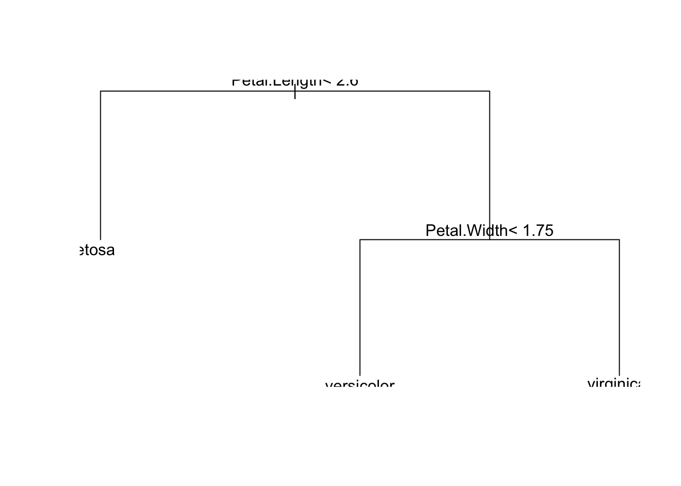

This gets cut off a bit, so let’s use some adjustments

# Plot the tree with adjusted margins
plot(ct_model, margin = 0.1)  # Increase the margin parameter for more space
text(ct_model,  cex = 0.8)

Explanation:

margin = 0.1: Adjusts the amount of white space around the tree. Increasing the margin will help ensure that the labels are not cut off.
cex = 0.8: Controls the size of the text labels. You can reduce the text size slightly to make sure everything fits well.

# Plot the tree with adjusted margins
plot(ct_model, margin = 0.1)  # Increase the margin parameter for more space
text(ct_model,  cex = 0.8)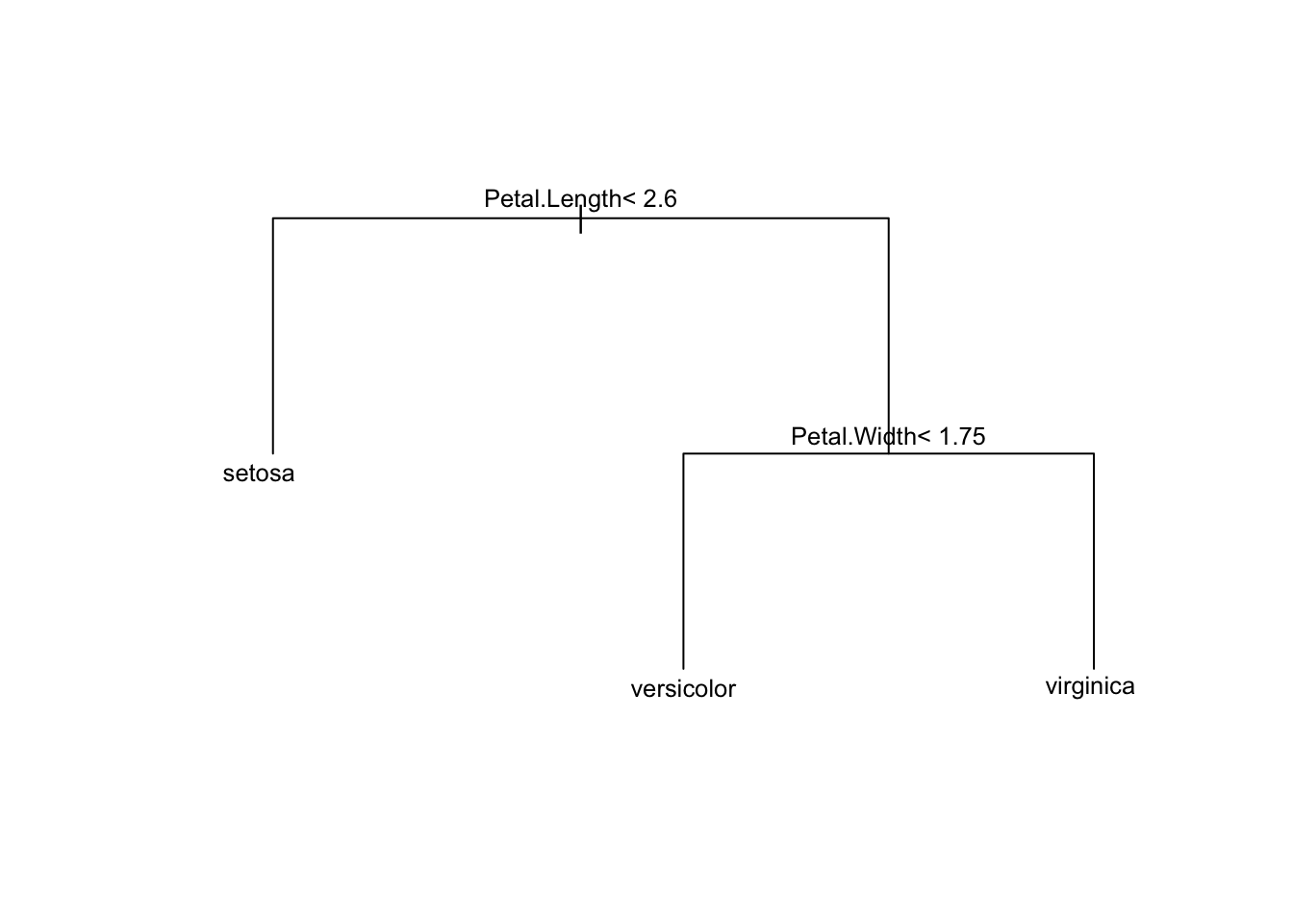

Note that the returned tree has already been pruned by default. More on this in the regression for CART section: Under-the-hood pruning

We can evaluate the CART Model by assessing its performance on predicting on the test set.

# Predict the species on the test data
predictions <- predict(ct_model, newdata = testData, type = "class")

# Evaluate the model with a confusion matrix
conf_matrix <- confusionMatrix(predictions, testData$Species)
print(conf_matrix)

Confusion Matrix and Statistics

            Reference
Prediction   setosa versicolor virginica
  setosa         15          0         0
  versicolor      0         14         2
  virginica       0          1        13

Overall Statistics
                                         
               Accuracy : 0.9333         
                 95% CI : (0.8173, 0.986)
    No Information Rate : 0.3333         
    P-Value [Acc > NIR] : < 2.2e-16      
                                         
                  Kappa : 0.9            
                                         
 Mcnemar's Test P-Value : NA             

Statistics by Class:

                     Class: setosa Class: versicolor Class: virginica
Sensitivity                 1.0000            0.9333           0.8667
Specificity                 1.0000            0.9333           0.9667
Pos Pred Value              1.0000            0.8750           0.9286
Neg Pred Value              1.0000            0.9655           0.9355
Prevalence                  0.3333            0.3333           0.3333
Detection Rate              0.3333            0.3111           0.2889
Detection Prevalence        0.3333            0.3556           0.3111
Balanced Accuracy           1.0000            0.9333           0.9167

In addition to providing the confusion matrix, the confusionMatrix() function provides some associated statistics; see ?confusionMatrix for details. We can see all these per class using:

stats_by_class <- conf_matrix$byClass
round(stats_by_class, 3) # round to read easier

                  Sensitivity Specificity Pos Pred Value Neg Pred Value
Class: setosa           1.000       1.000          1.000          1.000
Class: versicolor       0.933       0.933          0.875          0.966
Class: virginica        0.867       0.967          0.929          0.935
                  Precision Recall    F1 Prevalence Detection Rate
Class: setosa         1.000  1.000 1.000      0.333          0.333
Class: versicolor     0.875  0.933 0.903      0.333          0.311
Class: virginica      0.929  0.867 0.897      0.333          0.289
                  Detection Prevalence Balanced Accuracy
Class: setosa                    0.333             1.000
Class: versicolor                0.356             0.933
Class: virginica                 0.311             0.917

Multi-class classification metrics

In a multi-class classification problem, there is a separate metric for each class because we treat each class as the “positive” class while considering all other classes as “negative.” This approach provides a detailed evaluation of the model’s performance for each individual class.

Example: calculating precision for versicolor

Precision, also known as the Positive Predictive Value (PPV), is calculated as:

\[ \text{Precision} = \frac{\text{True Positives}}{\text{True Positives} + \text{False Positives}} \]

It measures how many of the instances predicted as a specific class (e.g., “versicolor”) are actually that class.

conf_matrix$table

            Reference
Prediction   setosa versicolor virginica
  setosa         15          0         0
  versicolor      0         14         2
  virginica       0          1        13

In the case of versicolor:

True Positives (TP) for “versicolor”: The number of times “versicolor” was correctly predicted as “versicolor”. This is the value at the intersection of row “versicolor” and column “versicolor,” which is 14.
False Positives (FP) for “versicolor”: The number of times other classes were incorrectly predicted as “versicolor.” This is the sum of the values in the “versicolor” row excluding the true positive, which is 2 (from predicting “virginica” as “versicolor”; if we had predicted some setosa as virginica, these values would have contributed to the sum as well).

Hence,

\[ \text{Precision (versicolor)} = \frac{\text{True Positives}}{\text{True Positives} + \text{False Positives}} = \frac{14}{14+2} = \frac{14}{16} = 0.875 \]

Pruning

The rpart function performs cross-validation to determine the optimal tree size based on the cp (cross-complexity $\alpha$) parameter. The goal is to find the smallest tree with the lowest cross-validated error. You can visualize the cross-validated error as a function of the complexity parameter using plotcp(). This plot helps identify the optimal cp value.

# Plot the cross-validation results
plotcp(ct_model)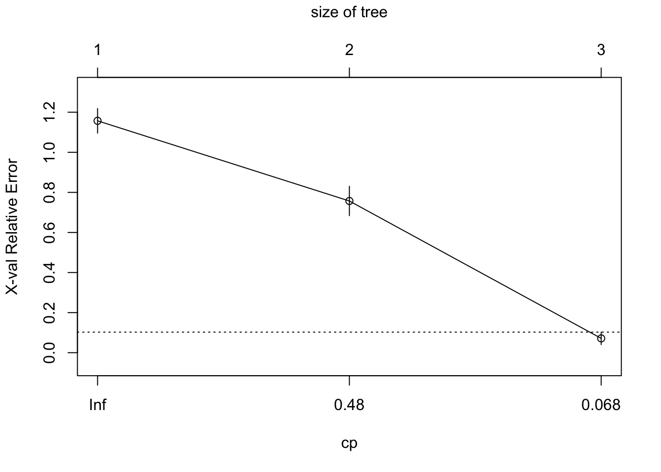

Alternatively we can access the table of numbers using:

# Display the CP table
printcp(ct_model)


Classification tree:
rpart(formula = Species ~ ., data = trainData, method = "class")

Variables actually used in tree construction:
[1] Petal.Length Petal.Width 

Root node error: 70/105 = 0.66667

n= 105 

       CP nsplit rel error   xerror     xstd
1 0.50000      0  1.000000 1.157143 0.061469
2 0.45714      1  0.500000 0.757143 0.073189
3 0.01000      2  0.042857 0.071429 0.031174

This output helps you understand how the cross-validated error changes as the tree size increases and help discern the optimal tree size. To obtain this programatically use:

# Prune the tree based on the optimal cp
optimal_cp <- ct_model$cptable[which.min(ct_model$cptable[,"xerror"]), "CP"]
optimal_cp

[1] 0.01

In our case, the optimal cp value is 0.01 which corresponds to our largest tree with 3 terminal nodes³. In our case this suggests we don’t need to prune our tree. If we did require pruning, we could easily achieve this using:

pruned_model <- prune(ct_model, cp = optimal_cp)

plot(pruned_model, margin = 0.1)  # Increase the margin parameter for more space
text(pruned_model,  cex = 0.8)

This doesn’t look any different from our first tree because, again, CV determined that our largest tree was optimal.

Regression Using CART

We will build a Regression Tree to predict the median house value (medv) in the Boston dataset based on various features such as crime rate, number of rooms, and distance to employment centers.

# Train a Regression Tree 
rt_model <- rpart(medv ~ ., data = train_boston, method = "anova")
rt_model

n= 356 

node), split, n, deviance, yval
      * denotes terminal node

 1) root 356 30280.05000 22.43539  
   2) rm< 6.974 307 12911.23000 19.93844  
     4) lstat>=14.4 128  2630.74300 14.92891  
       8) crim>=6.99237 56   817.18980 11.80179 *
       9) crim< 6.99237 72   840.01110 17.36111 *
     5) lstat< 14.4 179  4771.27400 23.52067  
      10) lstat>=5.41 156  2341.37200 22.47500  
        20) rm< 6.142 72   442.82440 20.67222 *
        21) rm>=6.142 84  1463.97600 24.02024  
          42) lstat>=10.04 27    89.49852 21.10741 *
          43) lstat< 10.04 57  1036.88000 25.40000 *
      11) lstat< 5.41 23  1102.38600 30.61304 *
   3) rm>=6.974 49  3462.44000 38.07959  
     6) rm< 7.437 27   728.38670 32.62222 *
     7) rm>=7.437 22   943.01860 44.77727 *

We can visualize the trained regression tree to better understand the decision rules and splits used to make predictions.

# Plot the regression tree
plot(rt_model, margin = 0.1)  # decrease margin for readability
text(rt_model, cex=0.8)       # decrease font size for readability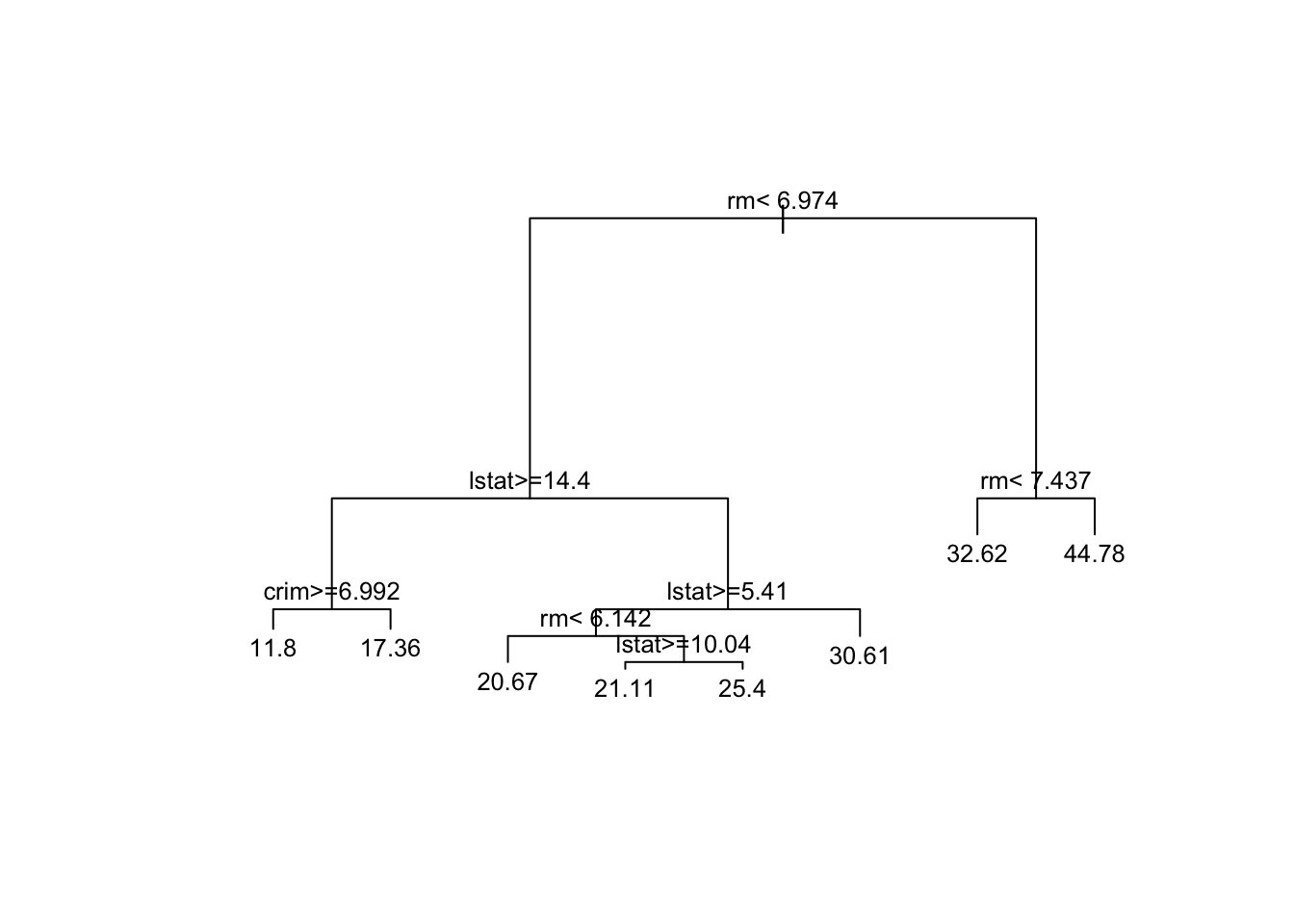

Let’s walk through an example prediction using the regression tree displayed. If a house had eight bedrooms (rm = 8)

Exercise 1 What would be the predicted median value a house with 8 bedrooms?

Click to show answer

The regression tree predicts a median house value of $44,780 according to my tree.

Exercise 2 What would be the predicted median value of a house with 3 rooms, an lstat of 15, and a crim of 8?

Click to show answer

The regression tree predicts a median house value of $11,800

Under-the-hood pruning

Note that the returned tree in rt_model has already been pruned by default. If you want to see what was going on under the hood, we can force rpart() to grow the “bushy” tree by setting the cost complexity $\alpha$ =0 (called cp)

bushy_tree <- rpart(
    formula = medv ~ .,
    data    = train_boston,
    method  = "anova", 
    control = list(cp = 0) # set the cost complexity parameter to 0 
)
plot(bushy_tree, margin = 0.1)  # decrease margin for readability
text(bushy_tree, cex=0.8)       # decrease font size for readability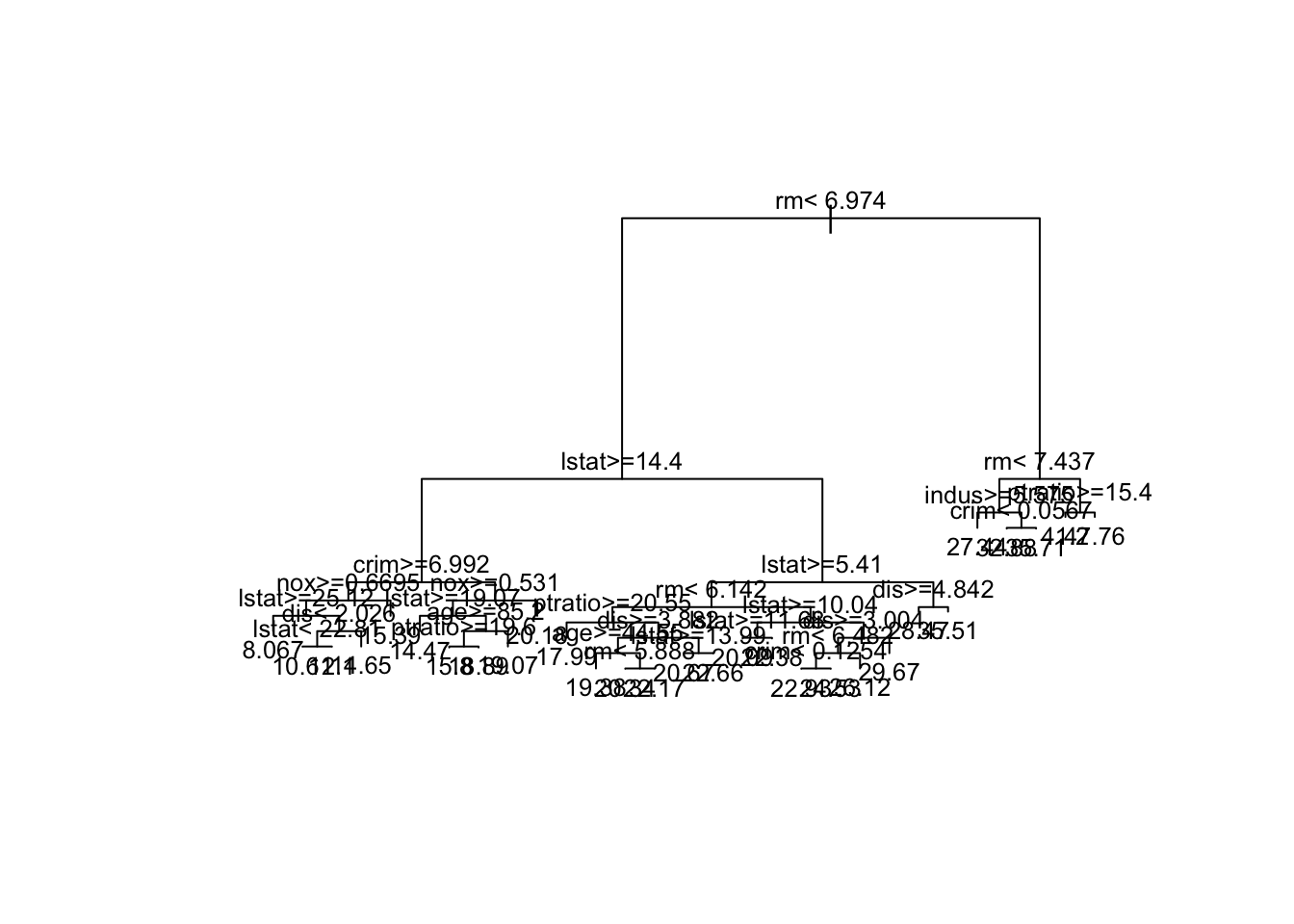

To see if pruning is needed let’s investigate the cross-validated error as a function of the complexity parameter

# Plot the cross-validation results
plotcp(bushy_tree)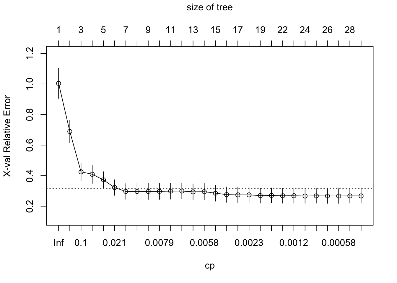

Figure 2 plot, produced by the plotcp() function, shows the cross-validated relative error (X-val Relative Error) as a function of the complexity parameter (cp) for different tree sizes in the regression tree. Here’s how to interpret the plot:

X-val Relative Error (Y-axis): This represents the relative error obtained during cross-validation. Lower values indicate a better fit to the data.
Tree Size (Top Axis): The top axis indicates the number of splits in the tree. The more splits, the larger the tree. For example, a tree size of 3 corresponds to a tree with three splits (four terminal nodes).
Complexity Parameter (cp, X-axis): cp controls the complexity of the tree. Smaller values of cp allow more splits, resulting in a larger tree. As cp decreases from left to right, the tree becomes more complex. We call this $\alpha$ in lecture.
Error Bars: The vertical lines through the circles represent one standard error above and below the relative error. The error bars help to identify a “simpler” tree using the “1-SE rule”: the smallest tree with an error within one standard error of the minimum error.
Dotted Line: The dotted line indicates the minimum cross-validated relative error plus one standard error. This is used in the “1-SE rule” to choose a tree size that balances error minimization and simplicity.

Although there are larger trees that obtain smaller errors (the optimal tree is the size of tree 0.0011025, 23, 0.1304064, 0.2664683, 0.0478719), after around 8 to 9 splits, the relative error levels off, and further reductions in cp lead to only small changes in the error. Breiman (1984) suggested that in actual practice, it’s common to instead use the smallest tree within 1 standard error (SE) of the minimum CV error (this is called the 1-SE rule).

bushy_tree$cptable

             CP nsplit rel error    xerror       xstd
1  0.4592590219      0 1.0000000 1.0041747 0.09848395
2  0.1819418775      1 0.5407410 0.6890487 0.07486655
3  0.0591489793      2 0.3587991 0.4251474 0.05765132
4  0.0438412339      3 0.2996501 0.4091417 0.05990402
5  0.0321512674      4 0.2558089 0.3723587 0.05358529
6  0.0143517729      5 0.2236576 0.3221754 0.05114942
7  0.0111491570      6 0.2093058 0.2966157 0.05119185
8  0.0083719806      7 0.1981567 0.2965119 0.05253017
9  0.0079829164      8 0.1897847 0.2968105 0.05257834
10 0.0077479872      9 0.1818018 0.2972195 0.05257129
11 0.0073025763     10 0.1740538 0.2987843 0.05256920
12 0.0072081108     11 0.1667512 0.2992372 0.05260494
13 0.0063130177     12 0.1595431 0.2941464 0.05259771
14 0.0053408420     13 0.1532301 0.2950650 0.05425578
15 0.0033841615     14 0.1478893 0.2854559 0.05251497
16 0.0024458345     15 0.1445051 0.2758200 0.05079462
17 0.0023382483     16 0.1420593 0.2742154 0.05054846
18 0.0023259169     17 0.1397210 0.2743393 0.04990572
19 0.0015136885     18 0.1373951 0.2692287 0.04880579
20 0.0015046350     20 0.1343677 0.2706268 0.04881435
21 0.0013104618     21 0.1328631 0.2683028 0.04881541
22 0.0011461897     22 0.1315526 0.2684987 0.04877251
23 0.0011025382     23 0.1304064 0.2664683 0.04787190
24 0.0006589333     24 0.1293039 0.2675239 0.04789028
25 0.0006129521     25 0.1286450 0.2668865 0.04796890
26 0.0005529878     26 0.1280320 0.2666654 0.04796618
27 0.0003346351     27 0.1274790 0.2673665 0.04797064
28 0.0000000000     28 0.1271444 0.2672827 0.04797088

More specifically, we’d choose the smallest tree where the error is within one standard error of the minimum error (above the dotted line). In this case, we could use a tree with 8 terminal nodes and reasonably expect to experience similar results within a small margin of error.

1-SE rule

The “1-SE rule,” will choose the smallest tree where the error is within one standard error of the minimum error (above the dotted line).

To prune using the 1-SE rule:

# Step 1: Find the minimum cross-validated error and its corresponding standard error
min_xerror <- min(bushy_tree$cptable[, "xerror"])
min_xstd <- bushy_tree$cptable[which.min(bushy_tree$cptable[, "xerror"]), "xstd"]

# Step 2: Calculate the threshold for the 1-SE rule
threshold <- min_xerror + min_xstd

# Step 3: Find the smallest tree where the xerror is within the threshold
# We use which() to find all indices where xerror is within the threshold
# Then we choose the smallest cp that satisfies this condition
optimal_cp_1se <- bushy_tree$cptable[which(bushy_tree$cptable[, "xerror"] <= threshold)[1], "CP"]

# Step 4: Prune the tree using the optimal cp from the 1-SE rule
pruned_model <- prune(bushy_tree, cp = optimal_cp_1se)

# Step 5: Plot the pruned tree
plot(pruned_model, margin = 0.1)
text(pruned_model, cex = 0.8)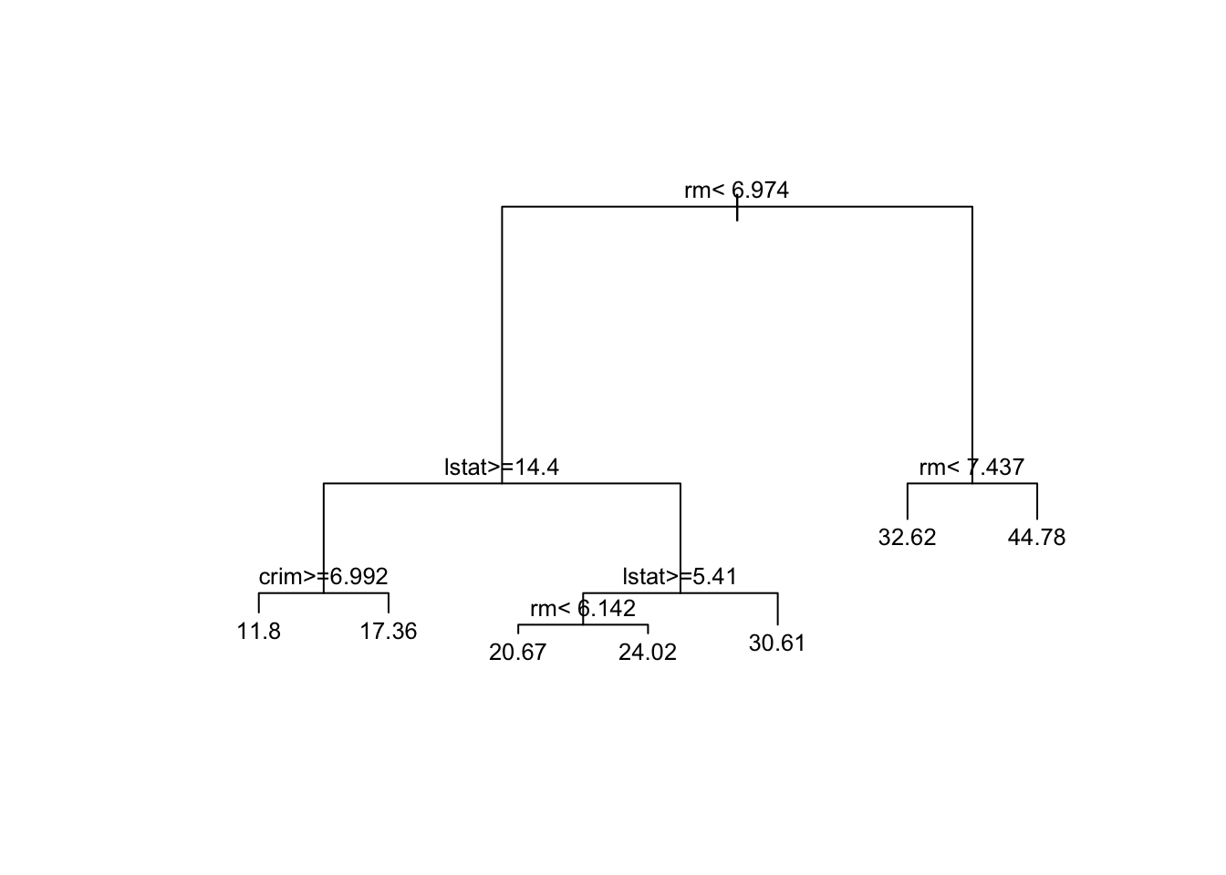

Notice that the pruned tree in Figure 3 is essentially the same as the tree obtained in Figure 1 when using the default settings; however, we achieve this result with significantly less effort. It’s worth noting that slight differences may appear due to the randomness introduced by the cross-validation process during the creation of the splits.

Evaluating the Regression Tree

Going back to the rt_model, we evaluate the regression tree’s performance by predicting on the test set and calculating metrics such as Mean Squared Error (MSE) and R-squared.

# Predict the median house value on the test data
predictions_reg <- predict(rt_model, newdata = test_boston)

# Calculate Mean Squared Error
mse <- mean((predictions_reg - test_boston$medv)^2)
mse

[1] 20.6667

The test Mean Squared Error, $MSE_{test}$, for the CART model is 20.6666971.

Bagging for Classification and Regression

Classification with Bagging (Random Forests)

# Train a random forest model for classification
rf_model <- randomForest(Species ~ ., data = trainData, 
                         ntree = 100, importance=TRUE)
rf_model


Call:
 randomForest(formula = Species ~ ., data = trainData, ntree = 100,      importance = TRUE) 
               Type of random forest: classification
                     Number of trees: 100
No. of variables tried at each split: 2

        OOB estimate of  error rate: 3.81%
Confusion matrix:
           setosa versicolor virginica class.error
setosa         35          0         0  0.00000000
versicolor      0         33         2  0.05714286
virginica       0          2        33  0.05714286

# Make predictions on the test set
rf_pred <- predict(rf_model, newdata = testData)

We can also look at variable importance from the bagging model (if we omit importance=TRUE) from the randomForest call, only the MeanDecreaseGini plot will be shown

varImpPlot(rf_model)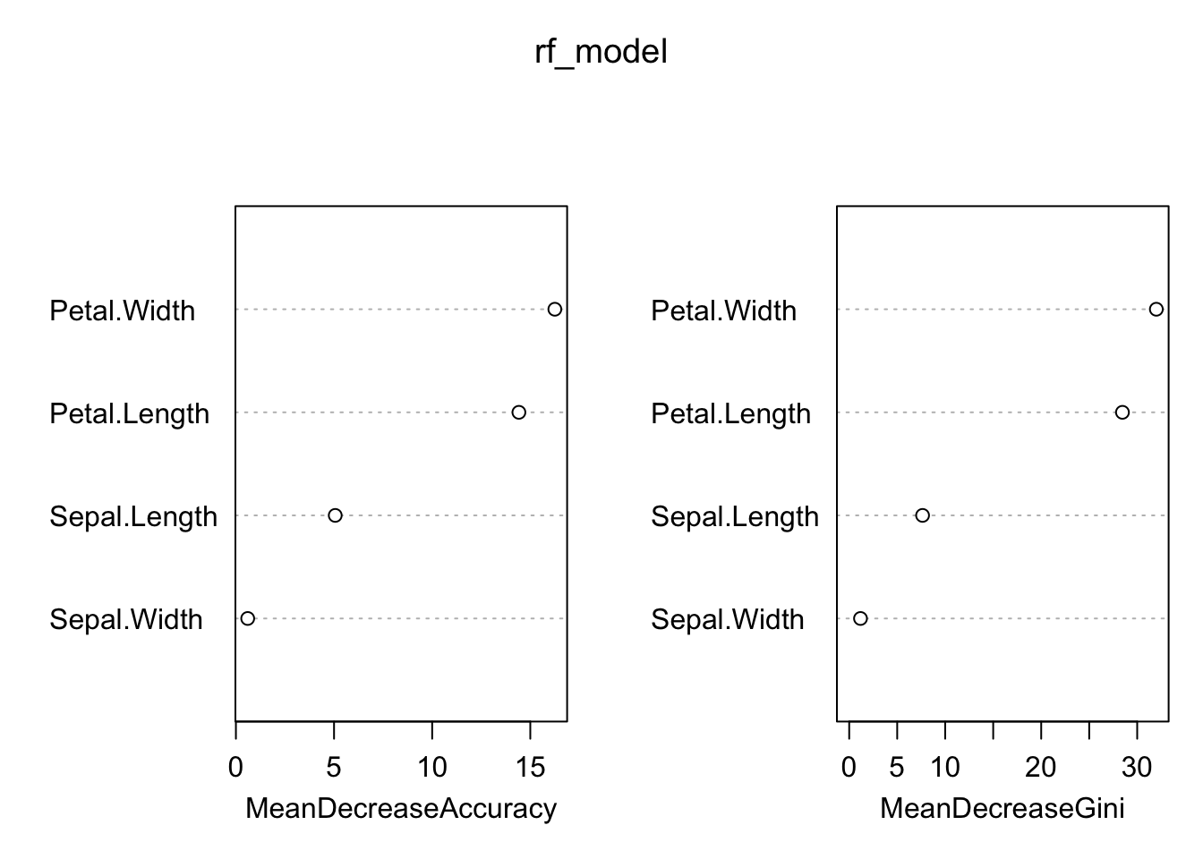

Based on Figure 4, Petal.Width and Petal.Length are the most important features for predicting the species of iris flowers, as indicated by both metrics.

We can evaluate the performance of this model using:

# Confusion matrix
rf_conf_mat = confusionMatrix(rf_pred, testData$Species)
rf_conf_mat

Confusion Matrix and Statistics

            Reference
Prediction   setosa versicolor virginica
  setosa         15          0         0
  versicolor      0         14         2
  virginica       0          1        13

Overall Statistics
                                         
               Accuracy : 0.9333         
                 95% CI : (0.8173, 0.986)
    No Information Rate : 0.3333         
    P-Value [Acc > NIR] : < 2.2e-16      
                                         
                  Kappa : 0.9            
                                         
 Mcnemar's Test P-Value : NA             

Statistics by Class:

                     Class: setosa Class: versicolor Class: virginica
Sensitivity                 1.0000            0.9333           0.8667
Specificity                 1.0000            0.9333           0.9667
Pos Pred Value              1.0000            0.8750           0.9286
Neg Pred Value              1.0000            0.9655           0.9355
Prevalence                  0.3333            0.3333           0.3333
Detection Rate              0.3333            0.3111           0.2889
Detection Prevalence        0.3333            0.3556           0.3111
Balanced Accuracy           1.0000            0.9333           0.9167

And the metrics by class:

rf_conf_mat$byClass

                  Sensitivity Specificity Pos Pred Value Neg Pred Value
Class: setosa       1.0000000   1.0000000      1.0000000      1.0000000
Class: versicolor   0.9333333   0.9333333      0.8750000      0.9655172
Class: virginica    0.8666667   0.9666667      0.9285714      0.9354839
                  Precision    Recall        F1 Prevalence Detection Rate
Class: setosa     1.0000000 1.0000000 1.0000000  0.3333333      0.3333333
Class: versicolor 0.8750000 0.9333333 0.9032258  0.3333333      0.3111111
Class: virginica  0.9285714 0.8666667 0.8965517  0.3333333      0.2888889
                  Detection Prevalence Balanced Accuracy
Class: setosa                0.3333333         1.0000000
Class: versicolor            0.3555556         0.9333333
Class: virginica             0.3111111         0.9166667

Regression with Bagging (Random Forests)

# Train a random forest model for regression
rf_model_reg <- randomForest(medv ~ ., data = train_boston, ntree = 100)
print(rf_model_reg)


Call:
 randomForest(formula = medv ~ ., data = train_boston, ntree = 100) 
               Type of random forest: regression
                     Number of trees: 100
No. of variables tried at each split: 4

          Mean of squared residuals: 11.30921
                    % Var explained: 86.7

# Make predictions on the test set
rf_pred_reg <- predict(rf_model_reg, newdata = test_boston)

# Calculate RMSE
mse_rf <- mean((rf_pred_reg - test_boston$medv)^2)

The test mean squared error $MSE_{test}$ for random forests on the Boston data is 12.2325484.

Boosting for Classification and Regression

Classification with Boosting (using `gbm`)

To perform classifcation with boosting :

# Train a boosting model
gbm_model <- gbm(Species ~ ., data = trainData, distribution = "multinomial",
                 n.trees = 100, interaction.depth = 3, shrinkage = 0.1, cv.folds = 5)

Warning: Setting `distribution = "multinomial"` is ill-advised as it is
currently broken. It exists only for backwards compatibility. Use at your own
risk.

summary(gbm_model)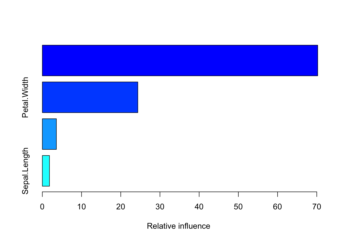

                      var   rel.inf
Petal.Length Petal.Length 70.244198
Petal.Width   Petal.Width 24.354908
Sepal.Width   Sepal.Width  3.582062
Sepal.Length Sepal.Length  1.818832

To evaluate our model lets test it on our training set:

# Make predictions on the test set
gbm_pred <- predict(gbm_model, newdata = testData, n.trees = 100, type = "response")
gbm_pred_class <- colnames(gbm_pred)[apply(gbm_pred, 1, which.max)]

# Confusion matrix
boost_reg_conf_mat = confusionMatrix(factor(gbm_pred_class), testData$Species)
boost_reg_conf_mat

Confusion Matrix and Statistics

            Reference
Prediction   setosa versicolor virginica
  setosa         15          0         0
  versicolor      0         14         2
  virginica       0          1        13

Overall Statistics
                                         
               Accuracy : 0.9333         
                 95% CI : (0.8173, 0.986)
    No Information Rate : 0.3333         
    P-Value [Acc > NIR] : < 2.2e-16      
                                         
                  Kappa : 0.9            
                                         
 Mcnemar's Test P-Value : NA             

Statistics by Class:

                     Class: setosa Class: versicolor Class: virginica
Sensitivity                 1.0000            0.9333           0.8667
Specificity                 1.0000            0.9333           0.9667
Pos Pred Value              1.0000            0.8750           0.9286
Neg Pred Value              1.0000            0.9655           0.9355
Prevalence                  0.3333            0.3333           0.3333
Detection Rate              0.3333            0.3111           0.2889
Detection Prevalence        0.3333            0.3556           0.3111
Balanced Accuracy           1.0000            0.9333           0.9167

For each species:

boost_reg_conf_mat$byClass

                  Sensitivity Specificity Pos Pred Value Neg Pred Value
Class: setosa       1.0000000   1.0000000      1.0000000      1.0000000
Class: versicolor   0.9333333   0.9333333      0.8750000      0.9655172
Class: virginica    0.8666667   0.9666667      0.9285714      0.9354839
                  Precision    Recall        F1 Prevalence Detection Rate
Class: setosa     1.0000000 1.0000000 1.0000000  0.3333333      0.3333333
Class: versicolor 0.8750000 0.9333333 0.9032258  0.3333333      0.3111111
Class: virginica  0.9285714 0.8666667 0.8965517  0.3333333      0.2888889
                  Detection Prevalence Balanced Accuracy
Class: setosa                0.3333333         1.0000000
Class: versicolor            0.3555556         0.9333333
Class: virginica             0.3111111         0.9166667

Regressions with boosting

# Train a boosting model for regression
gbm_model_reg <- gbm(medv ~ ., data = train_boston, distribution = "gaussian",
                     n.trees = 100, interaction.depth = 3, shrinkage = 0.1, cv.folds = 5)
summary(gbm_model_reg)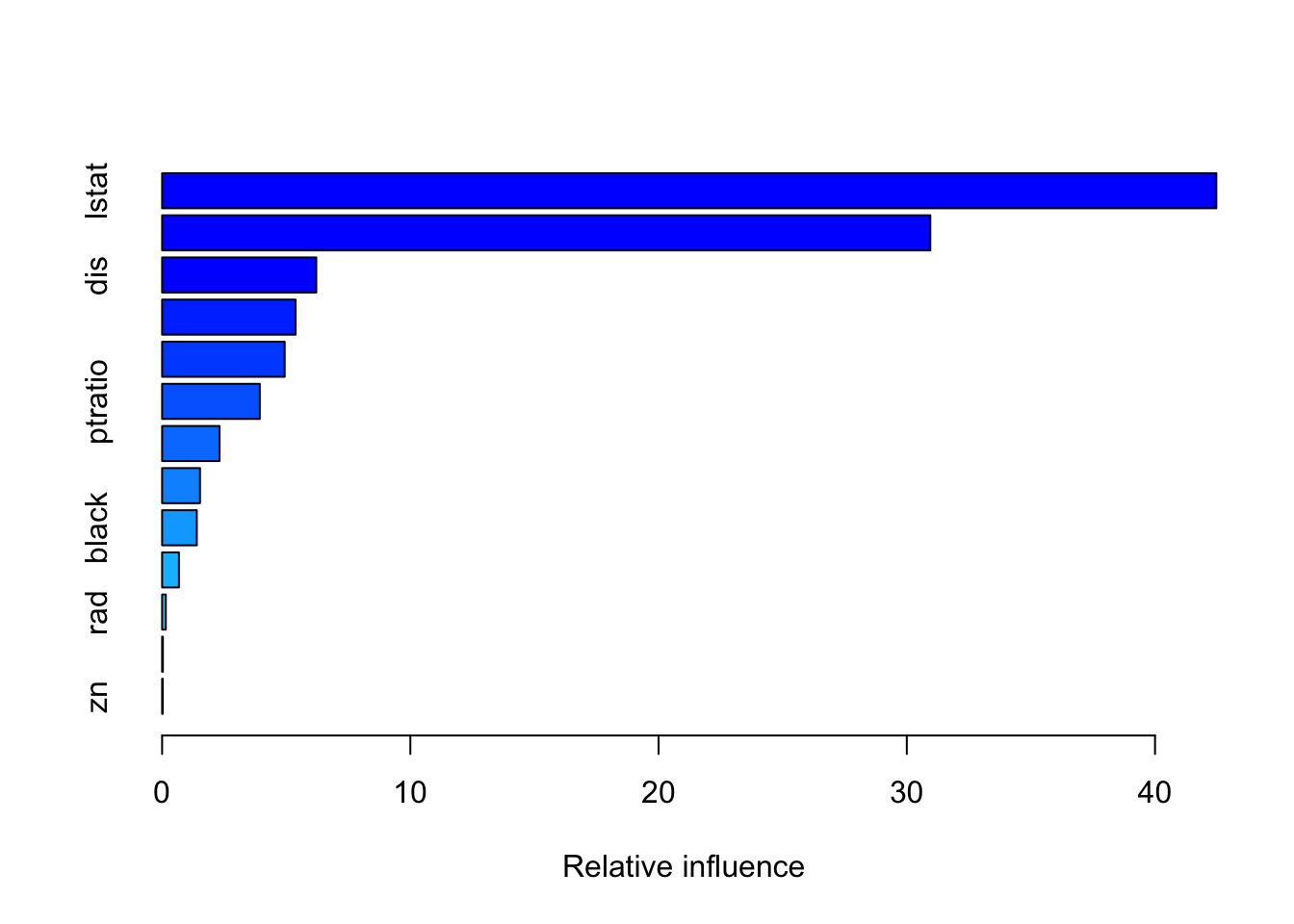

            var     rel.inf
lstat     lstat 42.47044834
rm           rm 30.94759835
dis         dis  6.21067532
crim       crim  5.37760515
nox         nox  4.93814113
ptratio ptratio  3.93501093
age         age  2.31365465
tax         tax  1.52643161
black     black  1.39738265
indus     indus  0.67658709
rad         rad  0.14883488
chas       chas  0.03092212
zn           zn  0.02670777

# Make predictions on the test set
gbm_pred_reg <- predict(gbm_model_reg, newdata = test_boston, n.trees = 100)

# Calculate RMSE
mse_gbm <- mean((gbm_pred_reg - test_boston$medv)^2)

The test MSE for the boosting model on the Boston data set is 12.850502.

Summary and Reflection

Comparison of Models:
- CART: It produces an interpretable model with a tree structure, making it easy to visualize decision rules. However, it may overfit the data unless pruned.
- Bagging (Random Forests): It reduces overfitting by aggregating many decision trees. The individual trees are less interpretable, but the overall model has improved predictive accuracy due to averaging.
- Boosting: It iteratively fits decision trees to the residuals of previous trees, enhancing model accuracy. However, it is more prone to overfitting if the learning rate and tree depth are not carefully tuned.
Impact of Parameters:
- ntree (number of trees): Increasing the number of trees generally enhances performance but may plateau after a certain point.
- shrinkage (learning rate): Smaller values increase training time but can improve accuracy by reducing the effect of each tree.
- interaction.depth: Higher values allow the model to capture more complex relationships but may increase the risk of overfitting.
Advantages and Limitations:
- CART: Simple and interpretable, but may not perform as well on complex datasets.
- Bagging: Better accuracy than CART but at the cost of model interpretability.
- Boosting: Can achieve the best accuracy but requires careful tuning and may be slower to train.

Other Resources

Chapter 9 Decision Trees. Hands on Machine Learning with R. Bradley Boehmke & Brandon Greenwell (2020). Taylor & Francis: https://bradleyboehmke.github.io/HOML/DT.html

Footnotes

the ranger package for example, maybe be preferable to randomForest if you are working with high dimensional data as it is much faster.↩︎
Reminder: the install.packages() command should be run in the R console, and should not be included in your .qmd script files.↩︎
the size of the tree (the number of terminal nodes) is given by nsplit + 1 where nsplit is the number of splits (nsplit in the outputted table).↩︎

Overview

Learning Objectives

Packages Required

Methods

CART

Random Forests

Boosting using gbm

Setup and Data Preparation

Iris Data set

Boston data set

Data Splitting

CART

Classification using CART

Pruning

Regression Using CART

Under-the-hood pruning

Evaluating the Regression Tree

Bagging for Classification and Regression

Classification with Bagging (Random Forests)

Regression with Bagging (Random Forests)

Boosting for Classification and Regression

Classification with Boosting (using gbm)

Regressions with boosting

Summary and Reflection

Other Resources

Footnotes

Boosting using `gbm`

Classification with Boosting (using `gbm`)