Cross-validation and the Bootstrap

Author

Dr. Irene Vrbik

Published

December 1, 2024

Introduction

In this lab, you will learn how to implement cross-validation and bootstrapping techniques in R to assess model performance and improve model robustness. These methods are essential for evaluating models beyond a single training set, helping to prevent overfitting and giving you more reliable estimates of model accuracy.

Goal: Learn how to perform k-fold cross-validation and leave-one-out cross-validation (LOOCV) to evaluate the performance of regression models. We will look at “by-hand” code and some functions from packages

R packages

Although these things are easy enough to code up by hand, we’ll be using some helpful pacakges to streamline the resampling and cross-validation approach.

carat package

The caret package (short for Classification And REgression Training) contains miscelleanous functions for training and plotting classification and regression models. For the detailed documentation visit: https://topepo.github.io/caret/. The current release version can be found on CRAN/caret and the project is hosted on github. Before we begin make sure you’ve installed the package using:

# Install caret if you haven't already 
install.packages("caret")

Recall, you should run this line directly in your console and you need only do it once. Each new session we will have to call and load the library using:

library(caret)

Loading required package: ggplot2

Loading required package: lattice

trainControl function

The trainControl() function in the caret package determines how the model training will be conducted. In this function we will need to specify the resampling method as either "boot" (for bootstraping), "cv" (for $k$-fold cross validation), "LOOCV" (for leave-one-out cross validation), or "none" (only fits one model to the entire training set). Note: there are more options that you can read about in the documentation; see ?trainControl

train function

The train() function

# General Syntax:

train(formula, data, method, trControl = NULL, tuneGrid = NULL, tuneLength = NULL, ...)

The main arguments are:

formula: The model formula (e.g., dist ~ speed for regression).
data: The dataset to be used for training.
method: The machine learning algorithm you want to use. For example, lm for linear regression, rf for random forests, knn for k-nearest neighbors, etc…¹
trControl: A list specifying the type of resampling or validation to use. This is created using the trainControl() function and can define cross-validation, bootstrapping, or other methods.
tuneGrid: A custom grid of hyperparameters that you can provide for tuning the model. This is particularly useful when you want to manually specify the values to try.
tuneLength: An integer that defines how many different values of the hyperparameters should be tested. If no tuneGrid is provided, tuneLength is used to automatically generate a range of values for tuning.
...: Additional arguments specific to the model.

createFolds function

The createFolds() function in the caret package is used to split your data into subsets or “folds” for the purpose of k-fold cross-validation. It creates indices that can be used to divide your dataset into training and testing subsets repeatedly, depending on how many folds you specify.

# Syntax
createFolds(y, k = 10, list = TRUE, returnTrain = FALSE)

The main arguments are:

y: A vector of data (usually the response variable or class labels) that is used to ensure stratified sampling. The function tries to create folds such that the proportion of different class labels or response values are roughly the same across all folds.
k: The number of folds (or subsets) you want to divide the data into. The default is k = 10, which creates 10 folds.
list: A logical value (default is TRUE) that specifies whether the output should be returned as a list. If list = TRUE, the function returns a list of indices for each fold. If list = FALSE, it returns a vector indicating the fold assignment for each observation.
returnTrain: A logical value (default is FALSE). If TRUE, the function returns the training set indices for each fold (i.e., all indices except the ones in that fold). If FALSE, it returns the test set indices for each fold.

Output:

When list = TRUE: The function returns a list where each element is a vector of indices corresponding to one fold. These indices can be used to subset your data for training or validation purposes.
When list = FALSE: The function returns a vector where each element corresponds to a fold assignment for each observation

boot package

The boot packages contains functions and datasets for bootstrapping from the book “Bootstrap Methods and Their Application” by A. C. Davison and D. V. Hinkley (1997, CUP), originally written by Angelo Canty for S. The current release version can be found on CRAN/boot. The documentation can be found here: https://cran.r-project.org/web/packages/boot/boot.pdf. It also contains handy functions and datasets for bootstrapping from the book Bootstrap Methods and Their Applicationby A. C. Davison and D. V. Hinkley (1997, CUP)

# Install caret if you haven't already 
install.packages("boot")

Recall, you should run this line directly in your console and you need only do it once. Each session, you’ll need to load the library before using any of its functions:

library(boot)


Attaching package: 'boot'

The following object is masked from 'package:lattice':

    melanoma

The cv.glm() function from the boot package in R is used to perform cross-validation for generalized linear models (GLMs), including ordinary linear models (lm). This function is versatile and can be used for different types of cross-validation, such as k-fold cross-validation and Leave-One-Out Cross-Validation (LOOCV), to estimate the predictive error of a model.

# General Syntax

cv.glm(data, glmfit, cost = function(y, yhat) mean((y - yhat)^2), K = n)

The main arguments are:

data: The data frame that contains the variables used in the model.
glmfit: The fitted model object created using the glm() function or lm() (since linear models are a special case of GLMs). This is the model on which cross-validation will be performed.
cost: This is a function that defines the cost function to be minimized. By default, the cost is the Mean Squared Error (MSE), but you can specify other loss functions depending on your needs.
K: The number of groups into which the data should be split to estimate the cross-validation prediction error². The default is to set K equal to the number of observations in data which gives the usual leave-one-out cross-validation.

The returned value is a list with the following components.

`call`	The original call to `cv.glm`.
`K`	The value of `K` used for the K-fold cross validation.
`delta`	A vector of length two. The first component is the cross-validation estimate of prediction error³.
`seed`	The value of `.Random.seed` when `cv.glm` was called.

Cars data

For a quick demo on how to do CV we will use the cars dataset from class. For simplicity, I will assume the entire cars data set makes up our training set so $n$ in this case is 50.

nrow(cars)

[1] 50

multiple cars data sets

The caret package also has a cars data set. We will be working with the cars data set from the datasets package (which comes preinstalled in R). If the cars dataset has been overwritten after loading the caret package, you can easily reload the original cars dataset from the datasets package using the following code:

data(cars, package = "datasets")

Linear Regression

LOOCV

Leave-one-out cross validation (LOOCV) is a special case of $k$-fold CV when $k =n$, the number of observations in our training set.

Manual coding

It’s relatively easy to set-up leave-one-out cross-validation yourself for any analysis. Here we can do it for the simple linear model…

# load the data set: specify the package to
# avoid confusion with the cars data from caret
data(cars, package = "datasets") 
attach(cars)
lm_loocv <- list()
mseloocv <- NA
for(i in 1:nrow(cars)){
  cvspeed <- speed[-i]
  cvdist <- dist[-i]
  lm_loocv[[i]] <- lm(cvdist ~ cvspeed)
  mseloocv[i] <- (predict(lm_loocv[[i]], newdata=data.frame(cvspeed=speed[i])) - dist[i])^2
}

# Calculate the CV MSE test
loocv_mse_slr = mean(mseloocv)
loocv_mse_slr

[1] 246.4054

\[MSE_{CV_{(n)}} = \frac{1}{n} \sum_{i=1}^n MSE_i = 246.4\]

Note: I am using slight different notation than lecture to distinguish between some other cross-validated metrics herein.

Using the caret package

Alternatively, this could be done using the caret package; see boot package section for general usage and syntax:

# Load necessary libraries
library(caret)

# Set up the trainControl function for LOOCV
control_loocv <- trainControl(method = "LOOCV")

# Run lm for LOOCV
lm_loocv <- train(dist ~ speed, data = cars, method = "lm", trControl = control_loocv)

# View results
lm_loocv

Linear Regression 

50 samples
 1 predictor

No pre-processing
Resampling: Leave-One-Out Cross-Validation 
Summary of sample sizes: 49, 49, 49, 49, 49, 49, ... 
Resampling results:

  RMSE      Rsquared   MAE     
  15.69731  0.6217139  12.05918

Tuning parameter 'intercept' was held constant at a value of TRUE

Notice that by default the regression metric don’t include the MSE. To calculate the CV MSE, we can simply square the CV RMSE:

# Extract RMSE from the model's results (this is the cross-validation RMSE)
rmse_loocv <- lm_loocv$results["RMSE"]

# Calculate MSE by squaring the RMSE
mse_loocv <- rmse_loocv^2
mse_loocv <- unname(mse_loocv) # remove the RMSE label
mse_loocv

          
1 246.4054

\[ MSE_{CV_{(n)}} = (RMSE_{CV_{(n)}})^2 = 246.405416^2 = 246.405416 \]

which, unsurprising, agrees with the one we calculated by hand. Recall: LOOCV is deterministic (i.e. not random) so we should get the same answer each time.

Using boot

You can also use the boot package to directly calculate cross-validation error (MSE) for an lm model. The cv.glm() function performs cross-validation and returns the MSE.

# Fit a linear model
lm_model <- glm(dist ~ speed, data = cars)
# the above is equivalent to 
# lm_model <- lm(dist ~ speed, data = cars)

# default K = n (so we can just leave K unspecified)
loocv_results <- cv.glm(cars, lm_model)  

# Extract the cross-validated MSE
loocv_mse <- loocv_results$delta[1]  # First value is the cross-validated MSE

# Print cross-validated MSE
loocv_mse

[1] 246.4054

Again, notice, that this estimate is consistent across each method (as it should be).

k-fold Cross-validation

For $k$-fold cross validation, the dataset is divided into $k$ parts/folds. At iteration 1, the first fold is used as the testing set and the remaining $k-1$ folds is used as the training set. The process is repeated $k$ times with each of the $k$ folds serving as the test set once. The out-of-sample performance, i.e. the performance metrics (e.g., accuracy, mean squared error, ROC-AUC) computed on each of the $k$ test sets, are averaged to produced the CV estimate.

semi-manual

While it would be relatively easy to code up $k$-fold CV validation ourselves, we can leverage the work of several packages to speed things up. For instance, in order to create $k$ folds we can use the createFolds() function from the caret package. For instance, if we wanted to do 5-fold cross validation:

# choose the number of folds
k = 5

# Create K folds
set.seed(123)  
folds <- createFolds(cars$speed,  # a vector of outcomes
                     k = k)       # the number of folds desired

The above will create k folds of indices from y = cars$speed. Each fold will contain indices for the data points that belong in the fold. We can view this using:

str(folds)

List of 5
 $ Fold1: int [1:9] 2 7 8 19 25 31 35 39 50
 $ Fold2: int [1:9] 1 3 9 18 26 34 36 41 45
 $ Fold3: int [1:12] 6 13 14 16 20 24 28 33 37 40 ...
 $ Fold4: int [1:11] 11 12 15 22 23 29 32 38 43 46 ...
 $ Fold5: int [1:9] 4 5 10 17 21 27 30 42 44

Here, folds$Fold1 will return the indices of the data points that are in the first fold, folds$Fold2 will give the second fold, and so on…

Next, we will train the model on each of the $k$ different training sets, where each set leaves out a single fold for testing. Note that folds[i] returns a list (even if it contains only one element). To convert this list into a simple vector of indices, we use unlist().

mse_values <- numeric(k)          # a vector to store MSEi's

for (i in 1:k) {
  train_indices <- unlist(folds[-i])  # Training indices
  test_indices <- unlist(folds[i])    # Test indices

  # Fit the model on the training set
  model <- lm(dist ~ speed, data = cars[train_indices,])
  # or we could have coded this up as:
  # model <- lm(dist ~ speed, data = cars subset = train_indices)
  
  # Make predictions on the test set
  predictions <- predict(model, newdata = cars[test_indices,])

  # Calculate the Mean Squared Error (MSE)
  mse_values[i] <- mean((cars$dist[test_indices] - predictions)^2)
}

# Cross-Validated MSE estimate:
(cv_mse_k5 <- mean(mse_values))

[1] 240.3434

For completion of the table below I’ve rerun the code with $k$=10 (hidden to save space and avoid repetition)

Code

k = 10

# Create K folds
set.seed(10)  
folds <- createFolds(cars$speed,  k = k)

mse_values <- numeric(k)       
for (i in 1:k) {
  train_indices <- unlist(folds[-i])  # Training indices
  test_indices <- unlist(folds[i])    # Test indices
  model <- lm(dist ~ speed, data = cars[train_indices,])
  predictions <- predict(model, newdata = cars[test_indices,])
  mse_values[i] <- mean((cars$dist[test_indices] - predictions)^2)
}

cv_mse_k10 <- mean(mse_values)

k-fold using the carat package

To perform k-fold cross-validation using the caret package, you can use the train() function, which simplifies the process of cross-validation for a wide variety of models. The trainControl() function allows you to specify the resampling method, such as k-fold cross-validation.

You can specify how many folds you want to use by setting the method to "cv" (for cross-validation) and setting number to the number of folds you want. We’ll use 5 and 10 for demonstration purposes (normally you can choose just one).

# Define the cross-validation method
control_5fold <- trainControl(method = "cv", number = 5)
control_10fold <- trainControl(method = "cv", number = 10)

Next we train the model with cross-validation using the train(). The example below uses a linear regression model (lm), but you can replace lm with other model types.

# Train the model using 5-fold cross-validation
set.seed(9894)
model5 <- train(dist ~ speed, data = cars, method = "lm", trControl = control_5fold)

# Train the model using 10-fold cross-validation
set.seed(1463)
model10 <- train(dist ~ speed, data = cars, method = "lm", trControl = control_10fold)

Switch up the seed

Notice how I use different seeds. Using different seeds in code when training models, such as in cross-validation, can help introduce variety into the random processes involved, such as partitioning data into folds, shuffling, or selecting subsets. If you use the same seed each time in your code, it will result in the same random sequence being generated for each operation that involves randomness.

The results will include the cross-validated performance of the model, such as the RMSE (Root Mean Squared Error) or other relevant metrics depending on the model. As before, we will convert these to CV MSE:

# Extract the cross-validation RMSE:
rmse_cv5 <- model5$results["RMSE"]
rmse_cv10 <- model10$results["RMSE"]

# Calculate MSE by squaring the RMSE
mse_cv5 <- unname(rmse_cv5^2)
mse_cv5

         
1 239.847

mse_cv10 <- unname(rmse_cv10^2)
mse_cv10

         
1 230.585

k-fold using the boot package

The cv.glm() function from the boot package calculates the estimated K-fold cross-validation prediction error for generalized linear models. Recall that these models have a shortcut formula so the model need only be fit once to obtain the CV estimates for MSE. To use the function we must first fit our regression model using glm()⁴:

The code is similar to that which we did in the LOOCV section above, only now, instead of using K = $n$ (default), we need to choose a reasonable value for K, see Note 1. For demonstration purposes, we’ll do 5-fold and 10-folds:

# Define the linear model
glm_model <- glm(dist ~ speed, data = cars)

# 5-fold cross-validation
set.seed(123)
cv_results_5 <- cv.glm(cars, glm_model, K = 5)
cv_results_10 <- cv.glm(cars, glm_model, K = 10)

Unlike LOOCV, the first value returned by delta is the cross-validated MSE:

cv_mse_5 <- cv_results_5$delta[1]  
cv_mse_5

[1] 244.1175

cv_mse_10 <- cv_results_10$delta[1]  
cv_mse_10

[1] 242.0437

Summary

All of the estimates summarized in the table below are estimating the same quantity: the MSE of the model when predicting new, unseen data. As discussed in class, LOOCV has lower bias but higher variance, while $k$-fold CV has a bit more bias but lower variance. This means that the $k$-fold estimate tends to be more stable (albeit slightly more biased⁵). As we can see, the estimates are all in the same ballpark, but they will differ notice how the $k$-fold runs will differ based on the random partitions into folds.

Cross-validated estimates of the MSE using LOOCV, and $k$ = 5, and 10.
Method	Manual	caret	boot
LOOCV	246.41	246.41	246.41
5-fold CV	240.34	239.85	244.12
10-fold CV	240.31	230.59	242.04

Note 1: Practical reccommendations for choosing the number of folds

5- or 10- fold CV is often preferred in practice. It’s computationally cheaper than LOOCV and tends to perform well in most situations.

KNN regression

Next we’ll do the same exercise for KNN. We’ll do this three ways: once using knn.reg(), once using caret. Note that the boot package is best suited for performing CV with linear models, so it is not appropriate here. Since KNN requires the tuning parameter of $k$ nearest neighbours (which will get confusing since we also use k to denote the number of folds!) we will also need to specify which values of $k$ to try. To be consistent with the previous section, lets try from 1 to 49. To avoid confusion between the two $k$’s well use k_folds and k_nn where possible.

LOOCV KNN

knn.reg

knn.reg() from the FNN package is another example of a function that has built-in (LOO) cross validation; see ?knn.reg. As described in the help file, if test is not supplied, Leave one out cross-validation is performed. Here we can make use of that to choose the number of nearest neighbours for KNN regression.

library(FNN)
kr <- list()
predmse <- NA

# the candidate values to try for our number of nearest neighbours
k_nn_vec = 1:49

for(i in k_nn_vec){
  kr[[i]] <- knn.reg(speed, test=NULL, dist, k=i)
  predmse[i] <- kr[[i]]$PRESS/nrow(cars)
}

plot(predmse, type="l", lwd=3, col="red")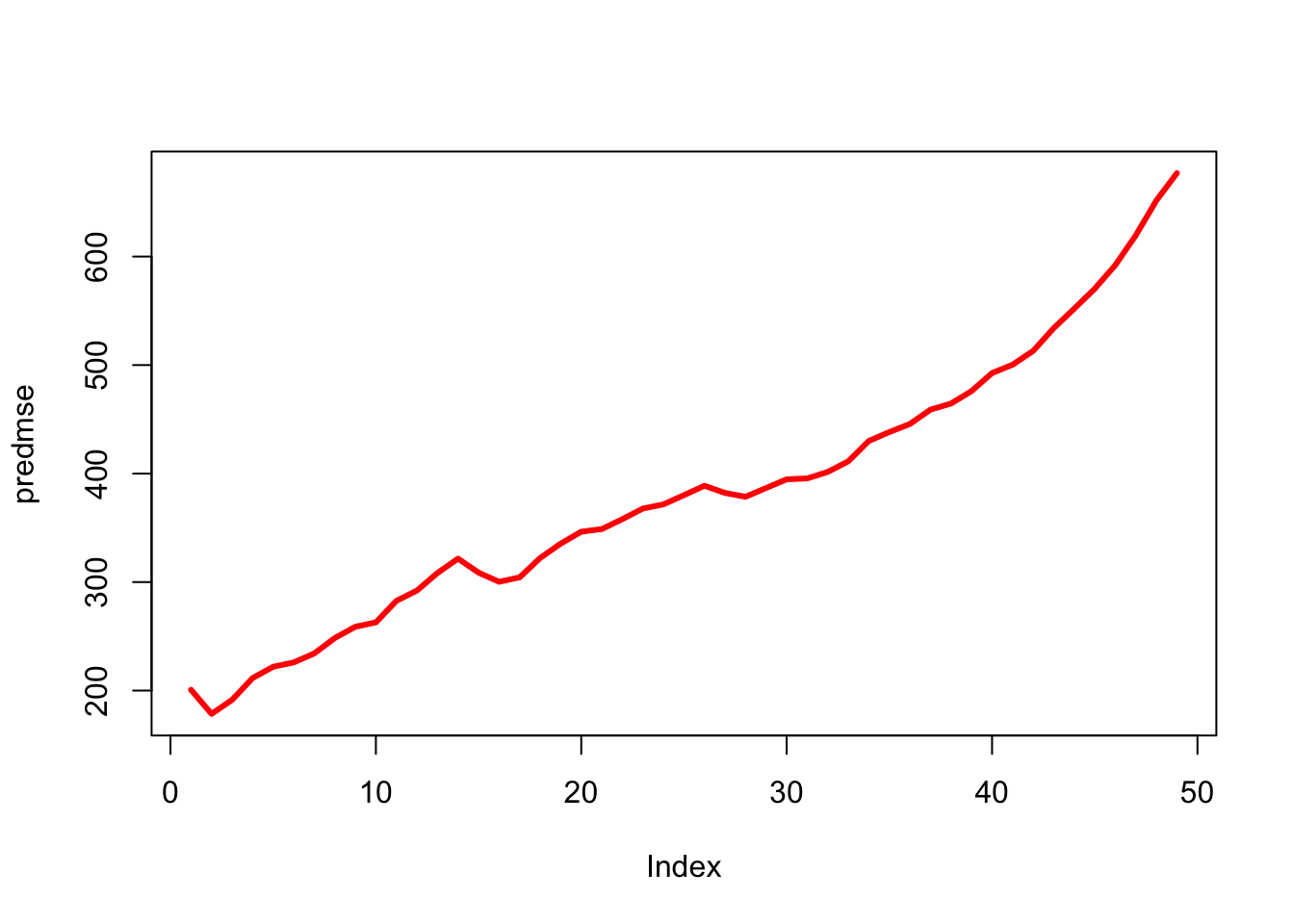

which.min(predmse)

[1] 2

plot(dist~speed)
seqx <- seq(from=0, to=30, by=0.01)
knnr <- knn.reg(speed, y=dist, test=matrix(seqx, ncol=1),  k=2) 
lines(seqx, knnr$pred, col="green", lwd=1)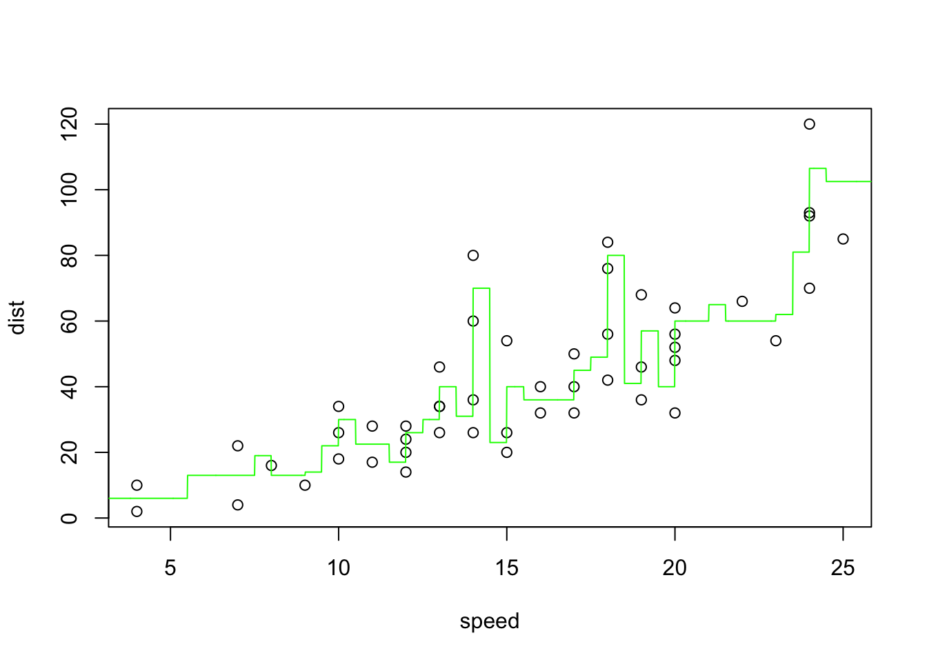

The CV MSE for the winning model is:

(mse_knn_reg = predmse[which.min(predmse)])

[1] 178.535

caret KNN

The code for this section is similar to the LOOCV in the linear regression section, only now, we need to switch the method from lm to knn .

# Set up training control using LOOCV
train_control <- trainControl(method = "LOOCV")

# Create a grid of k values from 1 to 49
k_grid <- expand.grid(k = 1:49)

# Define the model using k-NN
set.seed(123)
knn_model_loocv <- train(dist ~ speed, 
                         data = cars, 
                         method = "knn", 
                         trControl = train_control, 
                         tuneGrid = k_grid)   # Trying all k values from 1 to 49
# View the results (the best model is stroed as)
knn_model_loocv

k-Nearest Neighbors 

50 samples
 1 predictor

No pre-processing
Resampling: Leave-One-Out Cross-Validation 
Summary of sample sizes: 49, 49, 49, 49, 49, 49, ... 
Resampling results across tuning parameters:

  k   RMSE      Rsquared    MAE     
   1  17.22299  0.57771971  13.84900
   2  16.81462  0.59364378  13.03469
   3  16.32874  0.62188660  12.74524
   4  15.98970  0.60869934  12.27888
   5  15.79924  0.61692667  11.96067
   6  15.98720  0.60793955  12.26667
   7  16.84921  0.58456213  12.75144
   8  17.06976  0.56319622  13.03896
   9  16.85434  0.58027828  12.82896
  10  17.16124  0.56586393  13.27007
  11  17.37702  0.55581363  13.17682
  12  17.77312  0.54363718  13.30913
  13  17.73366  0.55443281  13.30204
  14  17.79687  0.55225609  13.39734
  15  17.93630  0.55212054  13.56614
  16  17.89203  0.55650024  13.48466
  17  18.22349  0.52581857  13.78783
  18  18.21679  0.52824000  13.73147
  19  19.06778  0.49151984  14.51179
  20  18.95363  0.49988875  14.44539
  21  18.94276  0.50118566  14.42743
  22  19.09070  0.49595241  14.68826
  23  19.03806  0.51229277  14.55499
  24  19.48921  0.48796762  14.75037
  25  19.59459  0.48054593  14.80893
  26  19.66843  0.48332166  14.97472
  27  19.76024  0.48379838  14.98436
  28  19.86830  0.48500253  15.09865
  29  20.08624  0.47776134  15.51675
  30  19.89567  0.49971544  15.38104
  31  20.86988  0.46895544  16.13642
  32  20.85333  0.47125698  16.08570
  33  20.85647  0.48008157  16.15815
  34  20.84894  0.48089403  16.13155
  35  21.71419  0.47208035  16.78270
  36  21.77776  0.46328199  16.93608
  37  21.76089  0.46493056  16.91877
  38  22.12245  0.44183983  17.31407
  39  22.46702  0.41400914  17.49862
  40  22.50325  0.40066240  17.64702
  41  22.91034  0.38323974  17.91136
  42  22.89386  0.38930235  17.91045
  43  23.04356  0.39556208  18.20231
  44  23.39353  0.36641378  18.51179
  45  24.92671  0.17613614  20.20738
  46  25.33215  0.04315454  20.53483
  47  25.35466  0.03169222  20.55194
  48  25.78441  0.36798681  20.82569
  49  26.03100  1.00000000  21.11918

RMSE was used to select the optimal model using the smallest value.
The final value used for the model was k = 5.

As displayed in the output, the best value of $k$ as chosen by cross validation is 5. You can get that answer programatically using:

# Extract the best k value
best_k_loocv <- knn_model_loocv$bestTune
cat("Best k (LOOCV):", best_k_loocv$k, "\n")

Best k (LOOCV): 5

Note that the final model that is trained using the best $k$ value is stored in the finalModel component. You can access it like this:

 knn_model_loocv$finalModel

5-nearest neighbor regression model

Hmm… we’re getting difference answers here than in LOOCV KNN. I’m not sure why that is… I will need to investigate this further.

Bonus mark for exam

The first person who can explain why the LOOCV results for KNN differ between the knn.reg and caret KNN implementation and correct the code so that the produce identical results (as I believe they should be) will get a bonus point on the final exam.

As before, we can get the cross-validated estimate of MSE by squaring the cross-validated estimate for RMSE. This can be achieved using:

# Extract cross-validated RMSE (Root Mean Squared Error)
win_index = which.min(knn_model_loocv$results$RMSE)
rmse_loocv <- knn_model_loocv$results$RMSE[win_index]

# Calculate MSE by squaring the RMSE
mse_loocv <- rmse_loocv^2
mse_loocv

[1] 249.6161

Finally let’s plot the original data and the fitted KNN model with the number of nearest neighbours as choose by CV:

plot(cars$speed, cars$dist, xlab = "Speed", ylab = "Distance", 
     main = paste("KNN Regression (k =", best_k_loocv, ")"))

# Make predictions using the best model
seqx <- seq(from=0, to=30, by=0.01)
newdata <- data.frame(speed = seqx)        
predictions <- predict(knn_model_loocv, newdata = newdata)
lines(seqx, predictions, col = "red", lwd = 2)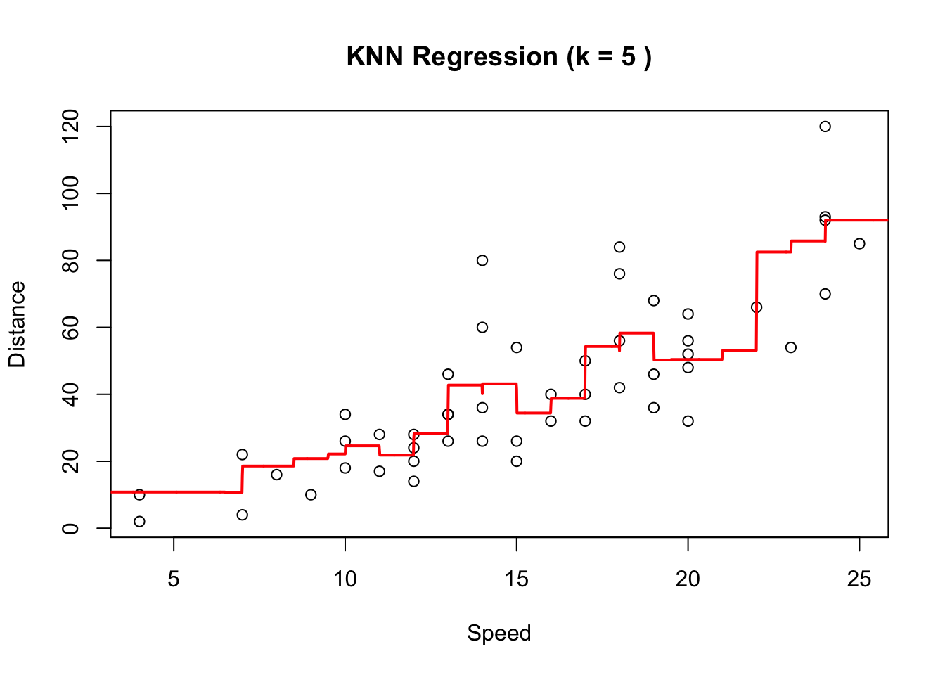

k-fold cross validation

When fitting KNN on the entire dataset, we initially considered the values from 1 through 49. This is no longer feasible for cross-validation because $k$ cannot exceed the number of points in the training set. When performing cross-validation (CV), each training set is smaller as it excludes the validation fold. Therefore, we’ll adjust the code to test from 1 up to 15.

knn.reg

To perform 5-fold cross-validation using knn.reg from the FNN package for k-Nearest Neighbors regression, you will need to manually set up the cross-validation process, as knn.reg does not have built-in cross-validation functionality like caret does.

As before, we will perform 5-fold and 10-fold cross-validation. If you’ve followed the examples above, the following code should be self-explanatory.

# Set up number of folds
k_folds <- 5

# Create K folds for cross-validation
set.seed(123)
folds <- createFolds(cars$speed, k = k_folds, list = TRUE)

# Initialize a matrix to store the MSE values for each k (1 to 49) across all folds
k_values <- 1:10
mse_matrix5 <- matrix(NA, nrow = k_folds, ncol = length(k_values))

# Loop through each value of k (number of neighbors) to perform cross-validation
for (k in k_values) {
  for (i in 1:k_folds) {
    # Get training and test indices
    train_indices <- unlist(folds[-i])
    test_indices <- unlist(folds[i])
    
    # Split the data into training and testing sets
    train_data <- cars[train_indices, ]
    test_data <- cars[test_indices, ]
    
    # Perform k-NN regression for this value of k
    # Convert the 'speed' column to matrix form to ensure knn.reg works correctly
    knn_model <- knn.reg(train = as.matrix(train_data$speed), 
                         test = as.matrix(test_data$speed), 
                         y = train_data$dist, k = k)
    
    # Calculate the MSE for this fold and store it
    mse_matrix5[i, k] <- mean((test_data$dist - knn_model$pred)^2)
  }
}

# Calculate the average MSE across all folds for each value of k
avg_mse_per_k5 <- colMeans(mse_matrix5, na.rm = TRUE)

# Find the optimal k (the one with the lowest MSE)
optimal_k5 <- which.min(avg_mse_per_k5)
cat("Optimal k:", optimal_k5, "\n")

Optimal k: 5

cv_mse_5fold = avg_mse_per_k5[optimal_k5]

# Print the MSE for the optimal k
cat("Cross-validated MSE for optimal k:", cv_mse_5fold, "\n")

Cross-validated MSE for optimal k: 265.2471

Again using 10-folds.

Code

# Set up number of folds
k_folds <- 10

# Create K folds for cross-validation
set.seed(123)
folds <- createFolds(cars$speed, k = k_folds, list = TRUE)

# Initialize a matrix to store the MSE values for each k (1 to 49) across all folds
mse_matrix10 <- matrix(NA, nrow = k_folds, ncol = length(k_values))

# Loop through each value of k (number of neighbors) to perform cross-validation
for (k in k_values) {
  for (i in 1:k_folds) {
    # Get training and test indices
    train_indices <- unlist(folds[-i])
    test_indices <- unlist(folds[i])
    
    # Split the data into training and testing sets
    train_data <- cars[train_indices, ]
    test_data <- cars[test_indices, ]
    
    # Perform k-NN regression for this value of k
    # Convert the 'speed' column to matrix form to ensure knn.reg works correctly
    knn_model <- knn.reg(train = as.matrix(train_data$speed), 
                         test = as.matrix(test_data$speed), 
                         y = train_data$dist, k = k)
    
    # Calculate the MSE for this fold and store it
    mse_matrix10[i, k] <- mean((test_data$dist - knn_model$pred)^2)
  }
}

# Calculate the average MSE across all folds for each value of k
avg_mse_per_k10 <- colMeans(mse_matrix10, na.rm = TRUE)

# Find the optimal k (the one with the lowest MSE)
optimal_k10 <- which.min(avg_mse_per_k10)
cat("Optimal k:", optimal_k10, "\n")

Optimal k: 3

Code

cv_mse_10fold = avg_mse_per_k10[optimal_k10]

# Print the MSE for the optimal k
cat("Cross-validated MSE for optimal k:", cv_mse_10fold, "\n")

Cross-validated MSE for optimal k: 251.8796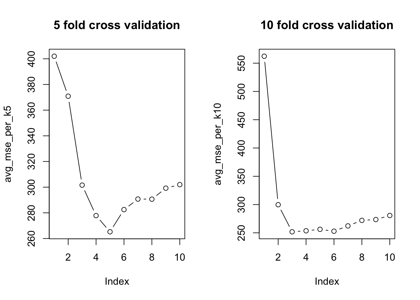

Notice how the optimal choice for $k$ differs from the 5-fold and 10-fold implementation; the former choose a $k$ nearest neighbour value of 5 and the latter, $k$ = 3

caret

To perform K-fold cross-validation and extract the MSE using caret, here’s how you can proceed:

# Set up training control for 5-fold cross-validation
set.seed(5023)
train_control <- trainControl(method = "cv", number = 5)

# Create a grid of k values from 1 to 30
k_grid <- expand.grid(k = 1:10)

# Define the model using k-NN
knn_model_cv <- train(dist ~ speed, 
                         data = cars, 
                         method = "knn", 
                         trControl = train_control, 
                         tuneGrid = k_grid)   

# Look at the results
knn_model_cv

k-Nearest Neighbors 

50 samples
 1 predictor

No pre-processing
Resampling: Cross-Validated (5 fold) 
Summary of sample sizes: 39, 39, 41, 41, 40 
Resampling results across tuning parameters:

  k   RMSE      Rsquared   MAE     
   1  17.82436  0.6099704  14.49827
   2  17.05437  0.6403416  13.52805
   3  16.40135  0.6662305  12.56247
   4  15.48093  0.6812195  11.45096
   5  14.96545  0.6773739  11.47145
   6  16.11588  0.6330477  12.64884
   7  15.84545  0.6504624  12.16476
   8  16.11074  0.6355928  12.58649
   9  16.57940  0.6005171  12.93264
  10  16.55728  0.6134936  12.70252

RMSE was used to select the optimal model using the smallest value.
The final value used for the model was k = 5.

# Extract the RMSE for the best model
win_index5 = which.min(knn_model_cv$results$RMSE)
best_rmse5 <- knn_model_cv$results$RMSE[win_index5]

# Convert RMSE to MSE
best_mse5 <- best_rmse5^2

# Print the cross-validated MSE
print(best_mse5)

[1] 223.9646

Do the same for 10-fold

Code

# Set up training control for 5-fold cross-validation
train_control <- trainControl(method = "cv", number = 5)

# Train KNN regression model using caret with cross-validation
knn_model <- train(dist ~ speed, 
                   data = cars, 
                   method = "knn", 
                   trControl = train_control, 
                    tuneGrid = k_grid)   

# Extract the RMSE for the best model
win_ind10 = which.min(knn_model$results$RMSE)
best_rmse10 <- knn_model$results$RMSE[win_ind10]

# Convert RMSE to MSE
best_mse10 <- best_rmse10^2

Summary

Below are the summary results from our experiments.

Method	knn.reg()	caret
LOOCV	178.535 (2 )	249.62 (5)
5-fold CV	265.25 (5)	223.96 (5)
10-fold CV	251.88 (3)	231.25 (5)

Notice how there is some discrepancy on the optimal value for $k$. See as how 5 appears the most often; I would be inclined to go with that.

Bootstrap Estimation

Manual

Here we will recreate the simulation provided in lecture for the nonparametric bootstrap

set.seed(311532)
x <- runif(30, 0, 1)
y <- 2*x + rnorm(30, sd=0.25)
mod1 <- lm(y~x)
newx <- list()
newy <- list()
modnew <- list()
coefs <- NA
for(i in 1:1000){
  #newx[[i]] <- runif(30, 0, 1)
  newx[[i]] <- x
  newy[[i]] <- 2*newx[[i]] + rnorm(30, sd=0.25)
  modnew[[i]] <- lm(newy[[i]]~newx[[i]])
  coefs[i] <- modnew[[i]]$coefficients[2]
}
set.seed(35134)
newboots <- list()
bootsmod <- list()
bootcoef <- NA
xy <- cbind(x,y)
for(i in 1:1000){
  newboots[[i]] <- xy[sample(1:30, 30, replace=TRUE),]
  bootsmod[[i]] <- lm(newboots[[i]][,2]~newboots[[i]][,1])
  bootcoef[i] <- bootsmod[[i]]$coefficient[2]
}

summary(mod1)$coefficients

               Estimate Std. Error     t value     Pr(>|t|)
(Intercept) -0.00427974 0.08754461 -0.04888639 9.613569e-01
x            2.05167004 0.12940570 15.85455727 1.620243e-15

sd(coefs)

[1] 0.1325126

sd(bootcoef)

[1] 0.132347

The theoretical standard error is 0.13735, so our hope is that all three values should be close to that. sd(coefs) (aside from the theoretical truth) would be a gold-standard approach for finding that value — but it is of course essentially impossible in practice to repeatedly gather new data. summary(mod1)$coefficients is based on the inferential linear regression assumptions (iid normal error, etc) and only one model fit. sd(bootcoef) is the bootstrap estimator based on resampling (with replacement) from the original sample.

As in class, we can push further by using the observed bootstrap estimators in bootcoef as an empirical distribution. First, we looked at the histogram

hist(bootcoef)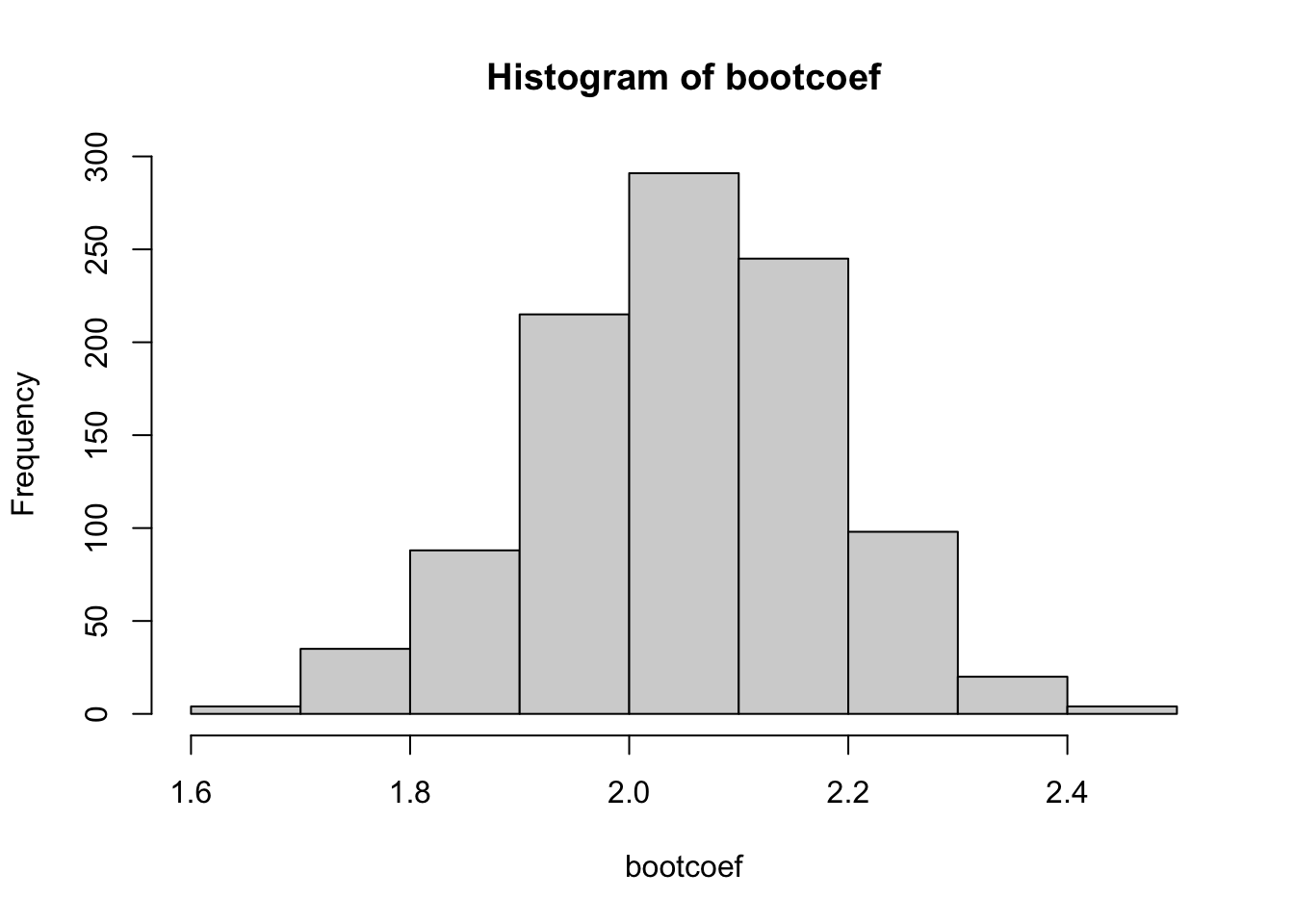

The simplest bootstrap confidence interval, often called Efron intervals (after the bootstrap founder Bradley Efron), simply pull the relevant percentiles of the observed bootstrap estimates.

So for example, for an approx 95% CI we would want the 2.5th and 97.5th percentiles of the observed estimates…

quantile(bootcoef, c(0.025, 0.975))

    2.5%    97.5% 
1.766970 2.296553

How about a 90% CI? Well, that would need the 5th and 95th percentiles

quantile(bootcoef, c(0.05, 0.95))

      5%      95% 
1.825115 2.261882

Notice that the true theoretical value (2.00) is contained within both of these intervals.

Using exisiting functions

Alternatively we could use existing packages like boot to automate the bootstrapping process. These packages provide functions that simplify the implementation and often support parallel processing for efficiency.

For example we could redo the above example using:

# Load the boot package
library(boot)

# Create a function to calculate the statistic of interest
beta_function <- function(data, indices) {
  sample_data <- data[indices,]
  fit <- lm(y~x, data = sample_data)
  return(coef(fit)["x"])
}

# Number of bootstrap samples
B <- 1000

# Set a seed for reproducibility
set.seed(6663492)

# Perform bootstrapping
dat <- data.frame(x, y)
boot_results <- boot(dat, beta_function, R = B)

# View the results
print(boot_results)


ORDINARY NONPARAMETRIC BOOTSTRAP


Call:
boot(data = dat, statistic = beta_function, R = B)


Bootstrap Statistics :
    original      bias    std. error
t1*  2.05167 0.002535141   0.1267117

Here beta_function() fits the linear regression model and pulls out the estimate for slope. More generally we will need to create a function that calculates our statistic (i.e. our function of our data, say, $T = t(X)$) out of resampled data. It should have at least two arguments: a data argument and an indices vector containing indices of elements from data that were picked to create a bootstrap sample.

boot_results have a few noteworthy outputs. $t contains the values our statistic $T(Z^{*j})$ where $Z^{*j}$ is the bootstrap sample and $j = 1, 2, \dots, B$:

head(boot_results$t)

         [,1]
[1,] 2.093083
[2,] 2.070167
[3,] 1.914885
[4,] 1.917636
[5,] 1.936294
[6,] 2.078371

hist(boot_results$t)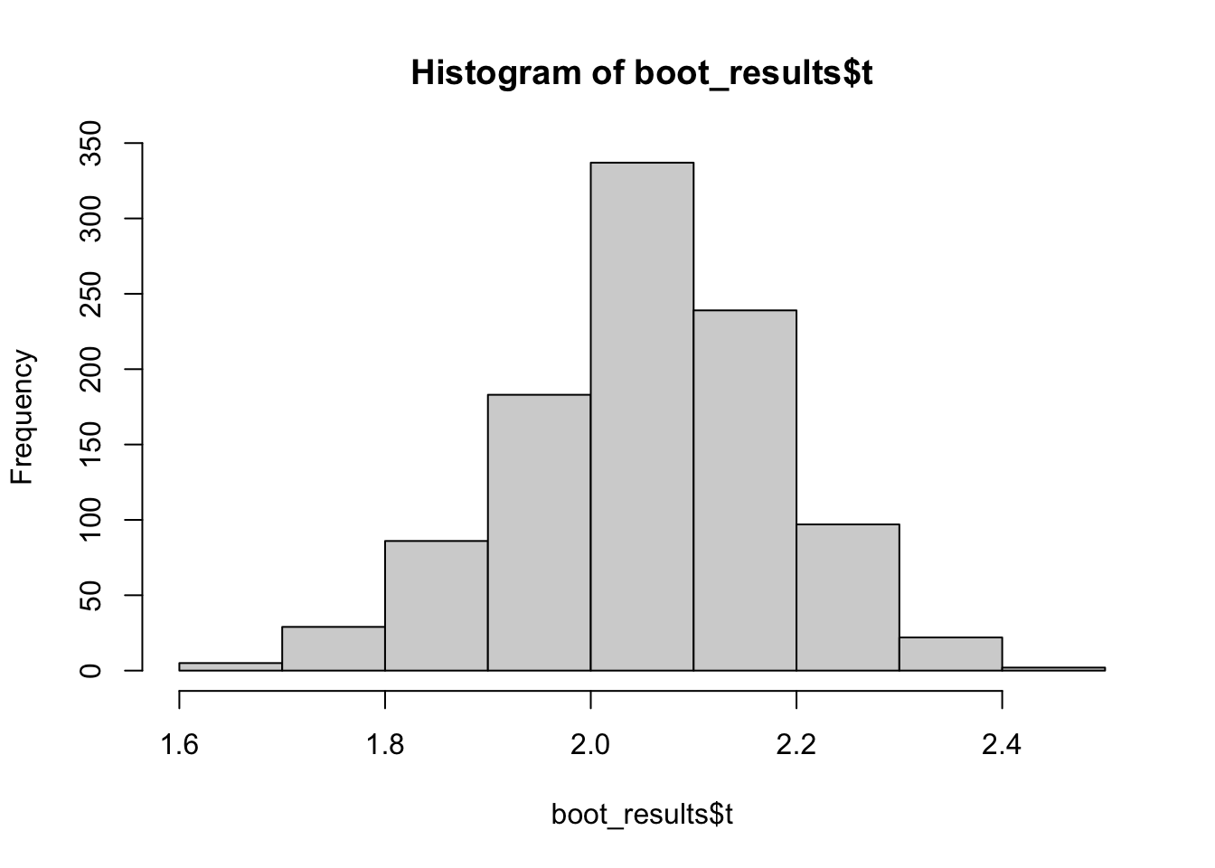

$t0 contains values of our statistic(s) in original, full, dataset:

full.fit <- lm(y~x, data = dat)
coef(full.fit)["x"]

      x 
2.05167

boot_results$t0 # same as above

      x 
2.05167

The Bootstrap Statistics:

original is the same as $t0
bias is a difference between the mean of bootstrap realizations (averge of $t values), and the value in original dataset (saved to $t0).
std. error is a standard error of bootstrap estimate, which equals standard deviation of bootstrap realizations.

sd(boot_results$t) # std.error in Bootstrap Statitiscs

[1] 0.1267117

Footnotes

Alternatively, you can use your one model in train() ; see https://topepo.github.io/caret/using-your-own-model-in-train.html ↩︎
The value of K must be such that all groups are of approximately equal size. If the supplied value of K does not satisfy this criterion then it will be set to the closest integer which does and a warning is generated specifying the value of K used.↩︎
We won’t discuss the second component, but in case you are interested, this is the adjusted cross-validation estimate. The adjustment is designed to compensate for the bias introduced by not using leave-one-out cross-validation.↩︎
When using glm() with the default settings of a Gaussian family and an identity link function (the default), it performs the same operation as lm() . Thus, glm(y ~ x, data) equivalent to lm(y ~ x, data) .↩︎
we did not discuss this in class, but the bias tends to be downward. i.e., we tend to underestimate MSE for new data and be overly optimist.↩︎