set.seed(23418)
x <- sort(runif(30,0,3))
y <- exp(x) + rnorm(length(x))
plot(x, y)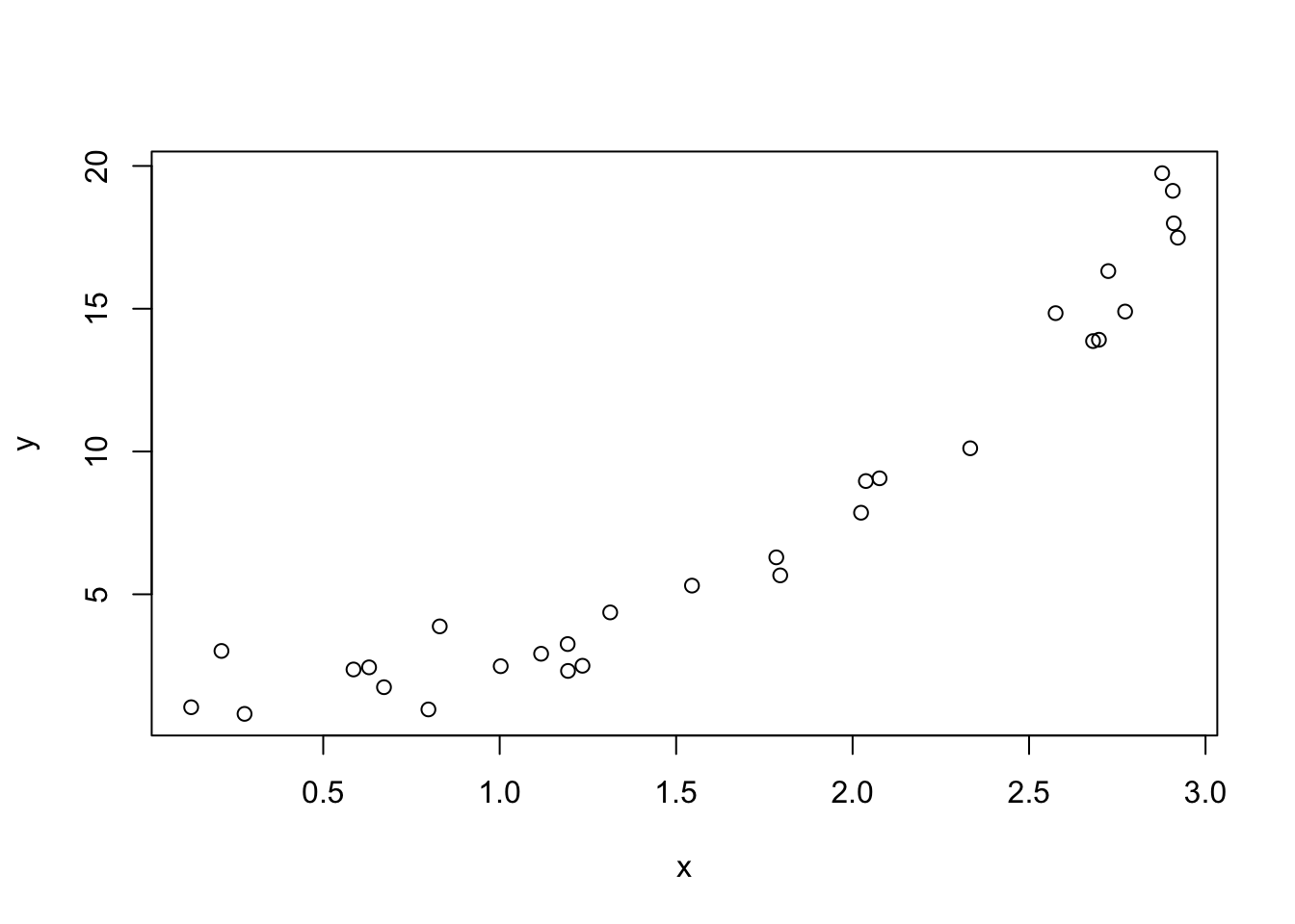
A look into the bias-variance tradeoff
Summary Throughout this lab, we will focus on evaluating the accuracy of supervised regression models using the Mean Squared Error (MSE). Specifically, we will cover the bias-variance trade-off and its implications on model flexibility, as well as the general trends between training MSE (\(MSE_{tr}\)) and test MSE (\(MSE_{Te})\).
Coverage - Topics roughly map to lecture 3, 4, and 5
Supplementary reading: For more, read 2.2 of the ISLR2 textbook.
By the end of this lab, you will be able to:
For reproducibility purpose, I have set a seed (set.seed()) for R’s random number generator. If you follow this code for creating these simulations your random numbers (and therefore subsequent images and calculations) should be identical1 to what I produced within this document.
Recall our general model for statistical learning \[\begin{equation}\label{eq:sl} Y = f(X) + \epsilon \end{equation}\]
where:
Our goal is to find an \(\hat f(X)\) that approximates the true function \(f(x)\) as well as possible. In this lab we will be discussing metrics for assessing model accuracy in the supervised setting. This corresponds to Section 2.2 of the ISLR2 textbook. By the end of it you should gain an understanding of the
For a continuous response variable, in the supervised setting, a natural measure of quality is how close our predict \(\hat y = \hat f (x)\) values compare to the “true” \(y\)s. In this context, the most commonly-used measure is the mean squared error (MSE). In words, the MSE is the average of all of the squared differences between the true values \(y_i\) and the the predicted values \(\hat f (x_i)\) (the smaller the better!).
When MSE is calculated using the training data \(\textbf{X}_{Tr} = \{(x_1, y_1),(x_2, y_2),...,(x_n, y_n)\} = \{x_i, y_i\}_{1}^n\) we call it the training MSE
\[MSE_{Tr} = \frac{1}{n} \sum_{i=1}^n (y_i-\hat f(x_i))^2\] When MSE is calculated using the testing data \(\textbf{X}_{Te} = \{(x_{n+1}, y_{n+1}),...,(x_{n+m}, y_{n+m})\} = \{x_i, y_i\}_{1}^m\) we call it the test MSE:
\[MSE_{Te} = \frac{1}{m} \sum_{i=1}^m (y_i-\hat f(x_i))^2\] where \(\hat f(x_i) = \hat y_i\) is the prediction for the \(i\)th input \(x_i\), and \(y_i\) is the response actually observed (ie “truth”).
Recall from lecture that we are more interested on how our models perform on the testing set rather than the training set. In other words we would like our models to perform well on data it has never “seen” before. Sometimes this is referred to as the generalisation performance. Models which obtain a lowest test MSE (as opposed to the lowest training MSE) are more desirable.
The bias-variance tradeoff is a fundamental characteristic shared by all (supervised) statistical learning models. It describes the interplay between how flexible the model is (variance of the model) and how well it performs on unseen data (bias of the model).
For a given test point \(x\), it can be shown2 that the expected test MSE, is given by: \[\begin{equation} \text{E}[(y - \hat f(x))^2] = \text{Var}(\hat f(x)) + (\text{Bias}[\hat f(x)])^2 + \text{Var}(\epsilon) \end{equation}\] That is, the reducible error in the MSE can actually be decomposed into two competing forces:
To get a sense of what is referred to as the bias-variance trade-off, let’s consider the contrived example in which we know what the true generating function \(f\) looks like. First, we’ll simulate our training data by uniformly generating \(X\) values, and then assuming an exponential relationship between \(X\) and \(Y\) with standard normal (mean 0, variance 1) errors. In other “words”, \[\begin{equation} Y = \exp(X) + \epsilon \end{equation}\] where \(\epsilon \sim \text{Normal}(\mu = 0, \sigma = 1)\).
set.seed(23418)
x <- sort(runif(30,0,3))
y <- exp(x) + rnorm(length(x))
plot(x, y)
Now fit a standard linear model, and add the fitted line (\(\hat f\)) to the plot in red:
linmod <- lm(y ~ x)
plot(x , y)
abline(linmod, col="red", lwd=2)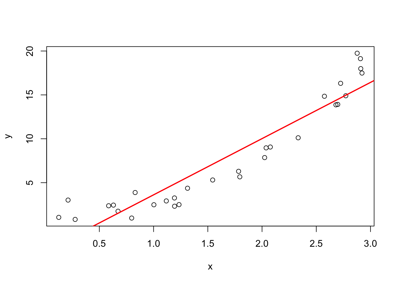
Next, we fit a local polynomial model using the loess function in R and add it in blue. We won’t delve into the specifics of this model3; instead, we’ll use it solely as an illustrative example of a relatively flexible model where the span argument controls the degree of smoothing. We we fit a local polynomial with medium flexibility (assigned to poly1 object) and one with high flexibility (which we’ll call poly2). The later approximately mimics the “connect-the-dots” scenario. N.B. you will get some errors when you fit this model (essentially warning us that this model is not reasonable) but just ignore them.
poly1 <- loess(y~x, span=0.75)
poly2 <- loess(y~x, span=0.1)
plot(x, y)
lines(x, predict(poly1), col="blue", lwd=3)
lines(x, predict(poly2), col="green", lwd=3)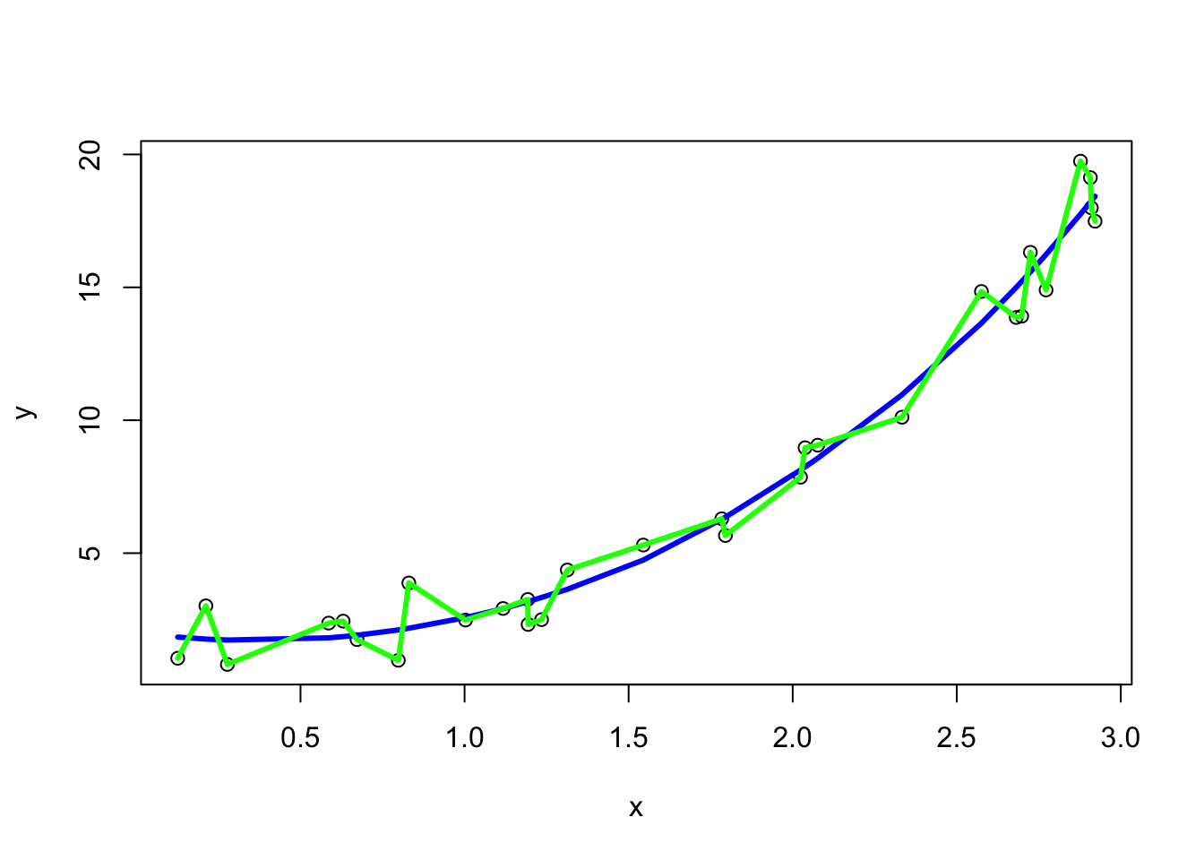
Now we can calculate the training MSE for each model by utilizing the predict() function. By default, predict() simply provides \(\hat{y}\) for a set of given \(x\)’s. To calculate the training MSE, we will provide the \(x\)’s used to train the model, i.e., we’ll use the predictors from the the training data. We’ll use round() to round the MSE to 2 decimal places.
# calculate the y^s for each model
yhat_lin <- predict(linmod)
yhat_poly1 <- predict(poly1)
yhat_poly2 <- predict(poly2)

# have a look at the first 6 predictions
# for the first 6 x's in our training data:
# x = training x (predictor)
# y = training y  (true response)
# yhat_* (predicted repsonse)
head(cbind(x, y, yhat_lin,yhat_poly1,yhat_poly2))
x y yhat_lin yhat_poly1 yhat_poly2
1 0.1257649 1.045191 -1.9872522 1.841613 1.045191
2 0.2116055 3.016159 -1.4372841 1.766126 3.016159
3 0.2770470 0.812518 -1.0180104 1.730300 0.812518
4 0.5857507 2.367584 0.9598088 1.813668 2.367584
5 0.6298887 2.441902 1.2425944 1.859171 2.441902
6 0.6721409 1.746828 1.5132979 1.910318 1.746828# calculate the training MSE
trmse_red <- mean((y - yhat_lin)^2)
trmse_blue <- mean((y - yhat_poly1)^2)
trmse_green <- mean((y - yhat_poly2)^2)
round(trmse_red, 2)
round(trmse_blue, 2)
round(trmse_green, 2)I have suppressed the output above and stored it in a table:
| Model | MSE\(_{train}\) |
|---|---|
| linear (red) | 4.37 |
| med flexibility (blue) | 0.83 |
| connect-the-dots (green) | 0 |
As expected, the connect-the-dots green model gets an \(MSE_{train}\) of zero.
Now we will simulate 10 new points from the same model to represent out training set. That is will generate some data that the fitting process didn’t “see” . We will plot them alongside our three fitted models:
set.seed(41368)
xnew <- sort(runif(10,0,3))
ynew <- exp(xnew) + rnorm(length(xnew))
plot(x, y)
abline(linmod, col="red", lwd=3)
lines(x, yhat_poly1, col="blue", lwd=3)
lines(x, yhat_poly2, col="green", lwd=3)
points(xnew, ynew, pch=15, col="purple", cex=1.5)
legend("topleft", col=c("red", "blue", "green", "purple"),
       pch = c(NA, NA, NA, 15), # Use NA for no point symbol
       lty = c(1,1,1,NA),       # Use NA for no line
       legend = c("Fitted simple linear model", "Fitted loess model with span = 0.75", "Fitted loess model with span = 1", "Test observations"),
       bty = "n" # Deleting this will put a box around the legend
       )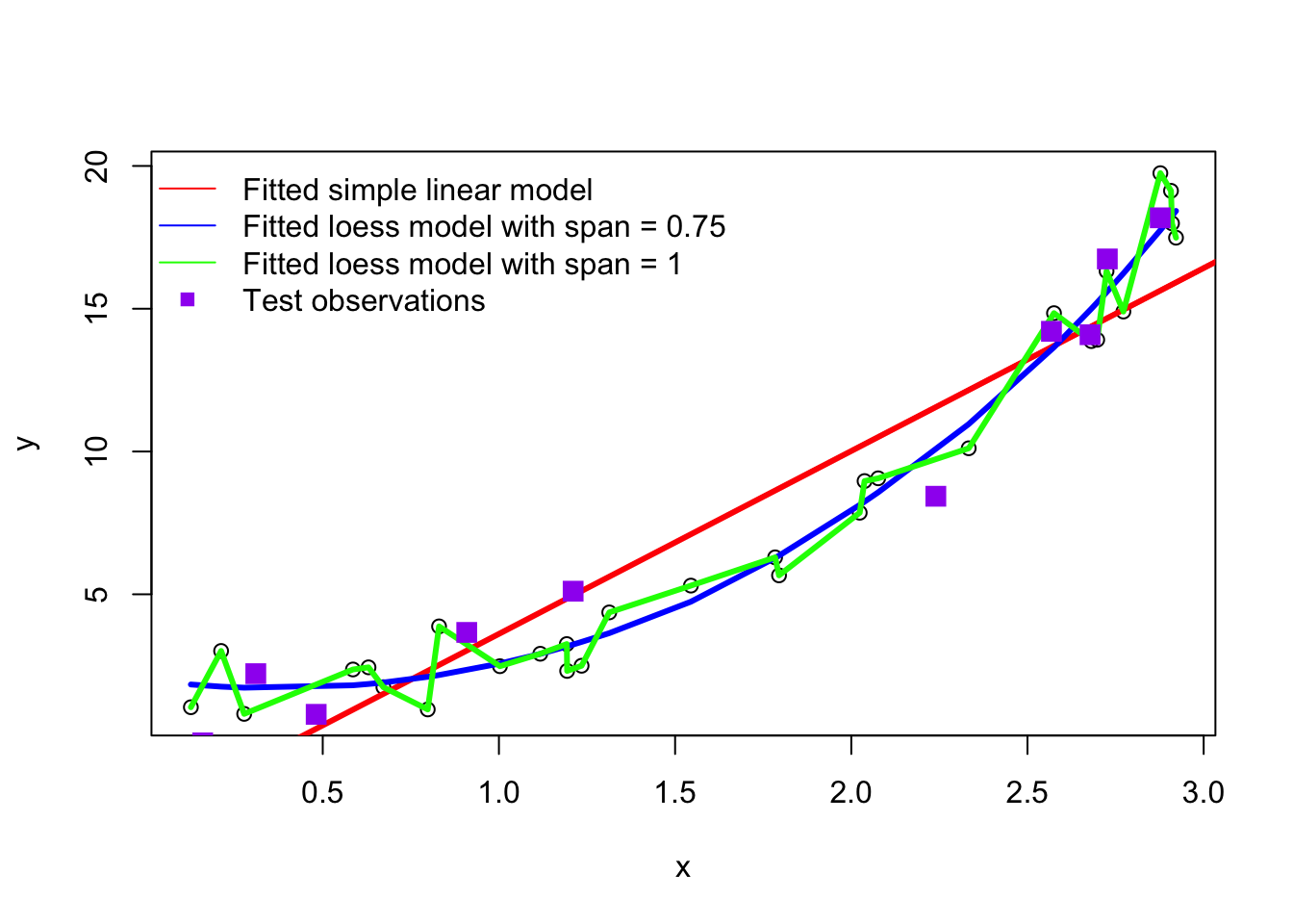
To calculate the test MSE we start by feeding the test observations (plotted in purple squares above) into the predict function. Note that predict specifically wants new data as a data.frame structure, and will not accept a vector object for newdata — we will run into little issues like this throughout the course.
# this will produce and error since xnew is not a data frame
# mean( (ynew - predict(linmod,  xnew)))^2

temse_red <- mean( (ynew - predict(linmod, data.frame(x = xnew)))^2 )
temse_blue <- mean( (ynew - predict(poly1, data.frame(x = xnew)))^2 )
temse_green <- mean((ynew - predict(poly2, data.frame(x = xnew)))^2 )
temse_red
temse_blue
temse_green| Model | MSE\(_{test}\) | MSE\(_{train}\) |
|---|---|---|
| linear (red) | 3.32 | 4.37 |
| med flexibility (blue) | 1.56 | 0.83 |
| connect-the-dots (green) | 4.29 | 0 |
We can see from the test MSE that the green more is not generalizable to new data points as it obtains the highest test MSE. Since the test MSE is much higher than the train MSE, we have a good indication that this model is overfitting. The red model obtains a similarly bad test and training MSE which is an indication that this model it too bias (i.e., underfitting). The blue model strikes a nice balance; it is neither too flexible, not too bias. As indicated by the MSE metrics, the \(MSE_{test}\) is not much worse that the \(MSE_{train}\).4 This provides some evidence that this model generalizes well to data it hasn’t seen.
Exercise Rerun this code with a different seed and see how the results change with additional simulations!
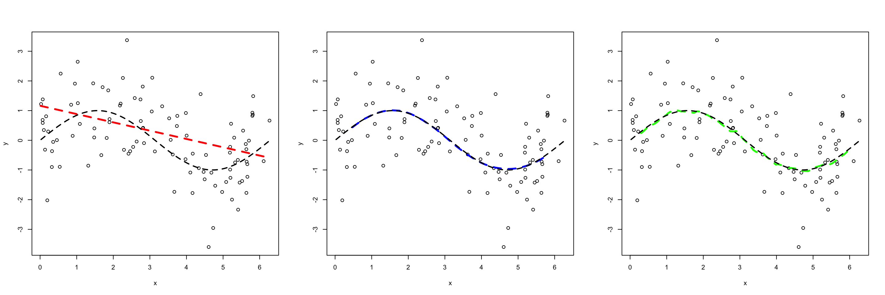
Next let’s simulate data by uniformly generating \(X\) values between 0 and 2\(\pi\), and generate \(Y\) values using: \[\begin{equation} Y = \text{sin}(X) + \epsilon \end{equation}\] where \(\epsilon \sim \text{Norm}(\mu =0, \sigma = 1)\). To get a sense of what “bias” and “variance” mean in the context of our fitted models, let’s look at fitted each model 100 different training sets. In the first figure we plot the first 10 fitted models, while the second figure plots the average prediction of each method over all of the 100 fitted models for a single test set \(X_{Te}\) (remember each fit was created using a different training set). Notice:
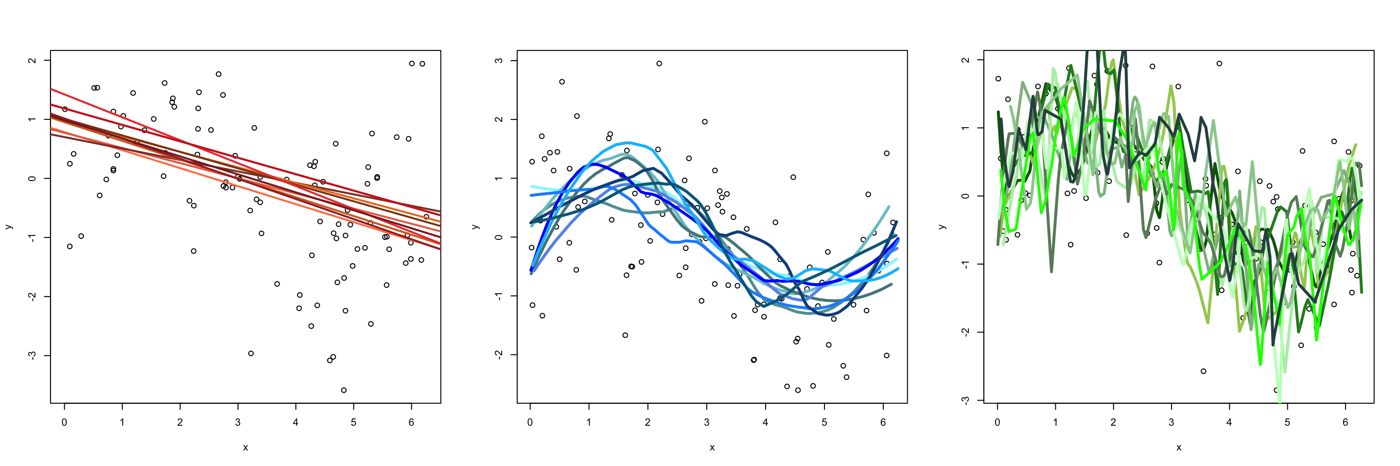
The green model (which is the most flexible) has the highest variability. This model is overfitting, that is, it follows the observations too closely. Thus a change in training set causes the estimate \(\hat f\) to change considerably. Notice that while the green model is highly variable, it has low bias. That is, even though a single fitted model does not close to our generating function \(f\), on average the estimate is close the truth.
In contrast, the red linear model (which is relatively inflexible) has low variance. That is to say, with each new training set it sees, the fitted model does not change much. While this model has low variance, it has high bias. Consequently, it will systematically underestimate/overestimate the true \(f\) (in black) for certain values of \(X\). For example, we can see in the figure below that between the range of \(x\) = 4 to 5 model is not capturing the “dip”, thus this model will systematically overestimate \(y\) in that region on average. This is a classic example of underfitting; no matter how much data this model learns from, it can never be persuaded away from a erroneous solution.
The blue model strikes a nice balance in between. It simultaneously has low variance and low bias.
Question Which of these models would you expect to have the lowest test MSE?
Recall the linear regression model takes the following form: \[\begin{equation} Y = \beta_0 + \beta_1 X_1 + \cdots + \beta_p X_p + \epsilon \end{equation}\] where:
Here are the simple and multiple linear regression models are fit on the life expectancy data; see ?state.x77 for details on this data set.
stdata <- data.frame(state.x77)
slr <- lm(stdata$Life.Exp~stdata$Illiteracy)
summary(slr)
mlr <- lm(stdata$Life.Exp~stdata$Illiteracy + stdata$Murder + stdata$HS.Grad + stdata$Frost)
summary(mlr)
stdata <- data.frame(state.x77) # convert the matrix to data.frame
# lm doesn't like periods in column names
#. you can quickly remove them using:
colnames(stdata) <- gsub("\\.", "", colnames(stdata))
slr <- lm(LifeExp~Illiteracy, data = stdata)
summary(slr)
Call:
lm(formula = LifeExp ~ Illiteracy, data = stdata)

Residuals:
    Min      1Q  Median      3Q     Max
-2.7169 -0.8063 -0.0349  0.7674  3.6675

Coefficients:
            Estimate Std. Error t value Pr(>|t|)
(Intercept)  72.3949     0.3383 213.973  < 2e-16 ***
Illiteracy   -1.2960     0.2570  -5.043 6.97e-06 ***
---
Signif. codes:  0 '***' 0.001 '**' 0.01 '*' 0.05 '.' 0.1 ' ' 1

Residual standard error: 1.097 on 48 degrees of freedom
Multiple R-squared:  0.3463,    Adjusted R-squared:  0.3327
F-statistic: 25.43 on 1 and 48 DF,  p-value: 6.969e-06
mlr <- lm(LifeExp~Illiteracy + Murder + HSGrad + Frost, data = stdata)
summary(mlr)
Call:
lm(formula = LifeExp ~ Illiteracy + Murder + HSGrad + Frost,
    data = stdata)

Residuals:
     Min       1Q   Median       3Q      Max
-1.48906 -0.51040  0.09793  0.55193  1.33480

Coefficients:
             Estimate Std. Error t value Pr(>|t|)
(Intercept) 71.519958   1.320487  54.162  < 2e-16 ***
Illiteracy  -0.181608   0.327846  -0.554  0.58236
Murder      -0.273118   0.041138  -6.639  3.5e-08 ***
HSGrad       0.044970   0.017759   2.532  0.01490 *
Frost       -0.007678   0.002828  -2.715  0.00936 **
---
Signif. codes:  0 '***' 0.001 '**' 0.01 '*' 0.05 '.' 0.1 ' ' 1

Residual standard error: 0.7483 on 45 degrees of freedom
Multiple R-squared:  0.7146,    Adjusted R-squared:  0.6892
F-statistic: 28.17 on 4 and 45 DF, p-value: 9.547e-12Before we begin with our working example, there are a few things we should point out about running a multiple linear regression model in R. Consider a data frame exdata which has columns Y, X, Z, and W. Then the following two fits are equivalen
fit1 <- lm(Y ~ ., data = D)
fit2 <- lm(Y ~ X + Z + W, data = exdata)
Similarly,
fit1 <- lm(Y ~ .-W, data = exdata) # is equivalent to
fit2 <- lm(Y ~ X + Z)
and
fit1 <- lm(Y ~ .*W, data = exdata) # is equivalent to
fit2 <- lm(Y ~ X + Z + W + X:W + Z:W)
If we want to call our variables without specifying the data, we would need to ``attach” the dataset first.
exdata <- data.frame(X=runif(5), Y=runif(5), Z=runif(5))
# X  <- will return return an error
attach(exdata)
X
[1] 0.599063127 0.424703312 0.547005700 0.338619425 0.005409968Now to our example from class. Consider the data set concerning the Life Expectancy rates for all 50 states from the 1970’s. For more information on this data set, type:
?state.x77We have seen a few model fits for this data in class, namely:
data(state)
# renames the rows to 2-letter abbreviation of state names
statedata <- data.frame(state.x77,row.names=state.abb)
colnames(statedata) <- gsub("\\.", "", colnames(statedata))
attach(statedata)
fit1 <- lm(LifeExp~Illiteracy)
fit2 <- lm(LifeExp~Illiteracy+Murder+HSGrad+Frost)
Let’s take a look at the model regresses the response variable LifeExp (life expectancy) by all of the remaining variables: {}.
fit <- lm(LifeExp~., data = statedata)
summary(fit)
Call:
lm(formula = LifeExp ~ ., data = statedata)

Residuals:
     Min       1Q   Median       3Q      Max
-1.48895 -0.51232 -0.02747  0.57002  1.49447

Coefficients:
              Estimate Std. Error t value Pr(>|t|)
(Intercept)  7.094e+01  1.748e+00  40.586  < 2e-16 ***
Population   5.180e-05  2.919e-05   1.775   0.0832 .
Income      -2.180e-05  2.444e-04  -0.089   0.9293
Illiteracy   3.382e-02  3.663e-01   0.092   0.9269
Murder      -3.011e-01  4.662e-02  -6.459 8.68e-08 ***
HSGrad       4.893e-02  2.332e-02   2.098   0.0420 *
Frost       -5.735e-03  3.143e-03  -1.825   0.0752 .
Area        -7.383e-08  1.668e-06  -0.044   0.9649
---
Signif. codes:  0 '***' 0.001 '**' 0.01 '*' 0.05 '.' 0.1 ' ' 1

Residual standard error: 0.7448 on 42 degrees of freedom
Multiple R-squared:  0.7362,    Adjusted R-squared:  0.6922
F-statistic: 16.74 on 7 and 42 DF,  p-value: 2.534e-10
Let’s illustrate some of the methods for varaible selection
Since Area has the highest \(p\)-value, we start by removing it from the model:
bmod1 <- lm(LifeExp~.-Area, data=statedata)
summary(bmod1)
Call:
lm(formula = LifeExp ~ . - Area, data = statedata)

Residuals:
     Min       1Q   Median       3Q      Max
-1.49047 -0.52533 -0.02546  0.57160  1.50374

Coefficients:
              Estimate Std. Error t value Pr(>|t|)
(Intercept)  7.099e+01  1.387e+00  51.165  < 2e-16 ***
Population   5.188e-05  2.879e-05   1.802   0.0785 .
Income      -2.444e-05  2.343e-04  -0.104   0.9174
Illiteracy   2.846e-02  3.416e-01   0.083   0.9340
Murder      -3.018e-01  4.334e-02  -6.963 1.45e-08 ***
HSGrad       4.847e-02  2.067e-02   2.345   0.0237 *
Frost       -5.776e-03  2.970e-03  -1.945   0.0584 .
---
Signif. codes:  0 '***' 0.001 '**' 0.01 '*' 0.05 '.' 0.1 ' ' 1

Residual standard error: 0.7361 on 43 degrees of freedom
Multiple R-squared:  0.7361,    Adjusted R-squared:  0.6993
F-statistic: 19.99 on 6 and 43 DF,  p-value: 5.362e-11
The above is equivalent to using the following command:
fit <- update(fit, .~. - Area)We will continue our backwards selection method using the update() formula. Since Illiteracy has the highest \(p\)-value, we remove it from the model:
fit <- update(fit, .~. -Illiteracy)
summary(fit)
Call:
lm(formula = LifeExp ~ Population + Income + Murder + HSGrad +
    Frost, data = statedata)

Residuals:
    Min      1Q  Median      3Q     Max
-1.4892 -0.5122 -0.0329  0.5645  1.5166

Coefficients:
              Estimate Std. Error t value Pr(>|t|)
(Intercept)  7.107e+01  1.029e+00  69.067  < 2e-16 ***
Population   5.115e-05  2.709e-05   1.888   0.0657 .
Income      -2.477e-05  2.316e-04  -0.107   0.9153
Murder      -3.000e-01  3.704e-02  -8.099 2.91e-10 ***
HSGrad       4.776e-02  1.859e-02   2.569   0.0137 *
Frost       -5.910e-03  2.468e-03  -2.395   0.0210 *
---
Signif. codes:  0 '***' 0.001 '**' 0.01 '*' 0.05 '.' 0.1 ' ' 1

Residual standard error: 0.7277 on 44 degrees of freedom
Multiple R-squared:  0.7361,    Adjusted R-squared:  0.7061
F-statistic: 24.55 on 5 and 44 DF,  p-value: 1.019e-11
## equivalent to:
#bmod2b <- lm(LifeExp ~. - Area - Illiteracy, data = statedata)
#summary(bmod2b)Since Income has the highest \(p\)-value, we remove it from the model:
fit <- update(fit, .~. -Income)
summary(fit)
Call:
lm(formula = LifeExp ~ Population + Murder + HSGrad + Frost,
    data = statedata)

Residuals:
     Min       1Q   Median       3Q      Max
-1.47095 -0.53464 -0.03701  0.57621  1.50683

Coefficients:
              Estimate Std. Error t value Pr(>|t|)
(Intercept)  7.103e+01  9.529e-01  74.542  < 2e-16 ***
Population   5.014e-05  2.512e-05   1.996  0.05201 .
Murder      -3.001e-01  3.661e-02  -8.199 1.77e-10 ***
HSGrad       4.658e-02  1.483e-02   3.142  0.00297 **
Frost       -5.943e-03  2.421e-03  -2.455  0.01802 *
---
Signif. codes:  0 '***' 0.001 '**' 0.01 '*' 0.05 '.' 0.1 ' ' 1

Residual standard error: 0.7197 on 45 degrees of freedom
Multiple R-squared:  0.736, Adjusted R-squared:  0.7126
F-statistic: 31.37 on 4 and 45 DF,  p-value: 1.696e-12
Since Population has the highest \(p\)-value, we remove it from the model:
fit <- update(fit, .~. -Population)
summary(fit)
Call:
lm(formula = LifeExp ~ Murder + HSGrad + Frost, data = statedata)

Residuals:
    Min      1Q  Median      3Q     Max
-1.5015 -0.5391  0.1014  0.5921  1.2268

Coefficients:
             Estimate Std. Error t value Pr(>|t|)
(Intercept) 71.036379   0.983262  72.246  < 2e-16 ***
Murder      -0.283065   0.036731  -7.706 8.04e-10 ***
HSGrad       0.049949   0.015201   3.286  0.00195 **
Frost       -0.006912   0.002447  -2.824  0.00699 **
---
Signif. codes:  0 '***' 0.001 '**' 0.01 '*' 0.05 '.' 0.1 ' ' 1

Residual standard error: 0.7427 on 46 degrees of freedom
Multiple R-squared:  0.7127,    Adjusted R-squared:  0.6939
F-statistic: 38.03 on 3 and 46 DF,  p-value: 1.634e-12
Since all p-value are below 0.05 (which I have selected to be my threshold) we can stop here. Note that the removal of Population is somewhat subjective. Since the pvalue is very close to the cutoff of 0.05, we may want to consider including this variable if interpretation is aided. In other words, if the ultimate goal is prediction, we could have made our cutoff 0.10 or 0.15 instead of 0.05 which would mitigate the risk of missing important predictors.
Notice that moving from the full to the final model only led to a reduction of \(R^2\) from 0.736 to 0.713. Hence, the simiplier model (which removedo four predictors from our full model) causes only a minor reduction in fit.
The data can be downloaded here: https://irene.vrbik.ok.ubc.ca/quarto/machine-learning/data/clockauction.txt
dat <- read.delim("data/clockauction.txt", sep="\t")
head(dat)
Age Bidders Price
1 127 13 1235
2 115 12 1080
3 127 7 845
4 150 9 1522
5 156 6 1047
6 182 11 1979plot(dat)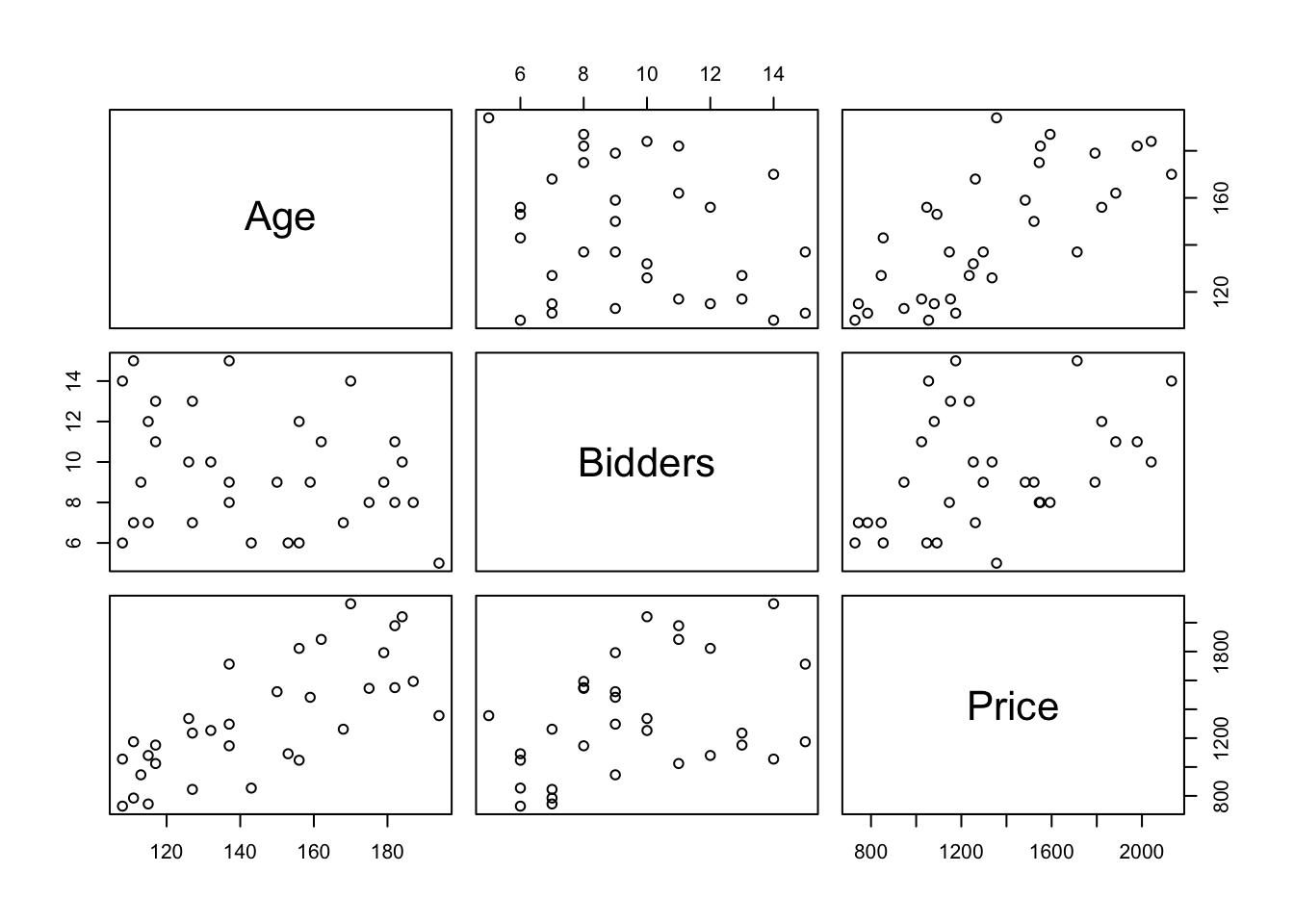
attach(dat)A simple linear regression model with age
agelm <- lm(Price~Age)
summary(agelm)
Call:
lm(formula = Price ~ Age)

Residuals:
    Min      1Q  Median      3Q     Max
-485.29 -192.66   30.75  157.21  541.21

Coefficients:
            Estimate Std. Error t value Pr(>|t|)
(Intercept)  -191.66     263.89  -0.726    0.473
Age            10.48       1.79   5.854  2.1e-06 ***
---
Signif. codes:  0 '***' 0.001 '**' 0.01 '*' 0.05 '.' 0.1 ' ' 1

Residual standard error: 273 on 30 degrees of freedom
Multiple R-squared:  0.5332,    Adjusted R-squared:  0.5177
F-statistic: 34.27 on 1 and 30 DF,  p-value: 2.096e-06
A simple linear regression model with bidders
bidlm <- lm(Price~Bidders)
summary(bidlm)
Call:
lm(formula = Price ~ Bidders)

Residuals:
    Min      1Q  Median      3Q     Max
-516.31 -355.27  -29.49  302.76  688.23

Coefficients:
            Estimate Std. Error t value Pr(>|t|)
(Intercept)   806.40     230.68   3.496  0.00149 **
Bidders        54.64      23.23   2.352  0.02540 *
---
Signif. codes:  0 '***' 0.001 '**' 0.01 '*' 0.05 '.' 0.1 ' ' 1

Residual standard error: 367.2 on 30 degrees of freedom
Multiple R-squared:  0.1557,    Adjusted R-squared:  0.1276
F-statistic: 5.534 on 1 and 30 DF,  p-value: 0.0254
A multiple linear regression model with age and bidders
ablm <- lm(Price~Age+Bidders); summary(ablm)
Call:
lm(formula = Price ~ Age + Bidders)

Residuals:
   Min     1Q Median     3Q    Max
-207.2 -117.8   16.5  102.7  213.5

Coefficients:
              Estimate Std. Error t value Pr(>|t|)
(Intercept) -1336.7221   173.3561  -7.711 1.67e-08 ***
Age            12.7362     0.9024  14.114 1.60e-14 ***
Bidders        85.8151     8.7058   9.857 9.14e-11 ***
---
Signif. codes:  0 '***' 0.001 '**' 0.01 '*' 0.05 '.' 0.1 ' ' 1

Residual standard error: 133.1 on 29 degrees of freedom
Multiple R-squared:  0.8927,    Adjusted R-squared:  0.8853
F-statistic: 120.7 on 2 and 29 DF,  p-value: 8.769e-15
A multiple linear regression model interaction between age and bidders
clm <- lm(Price~Age+Bidders + Age*Bidders); (sclm <- summary(clm))
Call:
lm(formula = Price ~ Age + Bidders + Age * Bidders)

Residuals:
     Min       1Q   Median       3Q      Max
-146.772  -70.985    2.108   47.535  201.959

Coefficients:
            Estimate Std. Error t value Pr(>|t|)
(Intercept) 322.7544   293.3251   1.100  0.28056
Age           0.8733     2.0197   0.432  0.66877
Bidders     -93.4099    29.7077  -3.144  0.00392 **
Age:Bidders   1.2979     0.2110   6.150 1.22e-06 ***
---
Signif. codes:  0 '***' 0.001 '**' 0.01 '*' 0.05 '.' 0.1 ' ' 1

Residual standard error: 88.37 on 28 degrees of freedom
Multiple R-squared:  0.9544,    Adjusted R-squared:  0.9495
F-statistic: 195.2 on 3 and 28 DF, p-value: < 2.2e-16library("gclus")Loading required package: clusterdata(body)
body$Gender <- factor(body$Gender)
# body$Gender[body$Gender==1] <- "Male"
# body$Gender[body$Gender==0] <- "Female"
simlm <- lm(Weight~Height, data=body)
multlm <- lm(Weight ~ Height + Gender, data=body)
intlm <- lm(Weight ~ Height*Gender, data=body)
summary(simlm)
Call:
lm(formula = Weight ~ Height, data = body)

Residuals:
    Min      1Q  Median      3Q     Max
-18.743  -6.402  -1.231   5.059  41.103

Coefficients:
              Estimate Std. Error t value Pr(>|t|)
(Intercept) -105.01125    7.53941  -13.93   <2e-16 ***
Height         1.01762    0.04399   23.14   <2e-16 ***
---
Signif. codes:  0 '***' 0.001 '**' 0.01 '*' 0.05 '.' 0.1 ' ' 1

Residual standard error: 9.308 on 505 degrees of freedom
Multiple R-squared:  0.5145,    Adjusted R-squared:  0.5136
F-statistic: 535.2 on 1 and 505 DF, p-value: < 2.2e-16summary(multlm)
Call:
lm(formula = Weight ~ Height + Gender, data = body)

Residuals:
    Min      1Q  Median      3Q     Max
-20.184  -5.978  -1.356   4.709  43.337

Coefficients:
             Estimate Std. Error t value Pr(>|t|)
(Intercept) -56.94949    9.42444  -6.043 2.95e-09 ***
Height        0.71298    0.05707  12.494  < 2e-16 ***
Gender1       8.36599    1.07296   7.797 3.66e-14 ***
---
Signif. codes:  0 '***' 0.001 '**' 0.01 '*' 0.05 '.' 0.1 ' ' 1

Residual standard error: 8.802 on 504 degrees of freedom
Multiple R-squared:  0.5668,    Adjusted R-squared:  0.5651
F-statistic: 329.7 on 2 and 504 DF, p-value: < 2.2e-16summary(intlm)
Call:
lm(formula = Weight ~ Height * Gender, data = body)

Residuals:
    Min      1Q  Median      3Q     Max
-20.187  -5.957  -1.439   4.955  43.355

Coefficients:
                Estimate Std. Error t value Pr(>|t|)
(Intercept)    -43.81929   13.77877  -3.180  0.00156 **
Height           0.63334    0.08351   7.584 1.63e-13 ***
Gender1        -17.13407   19.56250  -0.876  0.38152
Height:Gender1   0.14923    0.11431   1.305  0.19233
---
Signif. codes:  0 '***' 0.001 '**' 0.01 '*' 0.05 '.' 0.1 ' ' 1

Residual standard error: 8.795 on 503 degrees of freedom
Multiple R-squared:  0.5682,    Adjusted R-squared:  0.5657
F-statistic: 220.7 on 3 and 503 DF, p-value: < 2.2e-16plot(body$Height, body$Weight)
# plot the line for females
abline(a=intlm$coefficients[1], b=intlm$coefficients[2],col=1)
# plot the line for males
manslope <- intlm$coefficients[2] + intlm$coefficients[4]
manint <-intlm$coefficients[1] + intlm$coefficients[3]
abline(a=manint, b=manslope,col=2)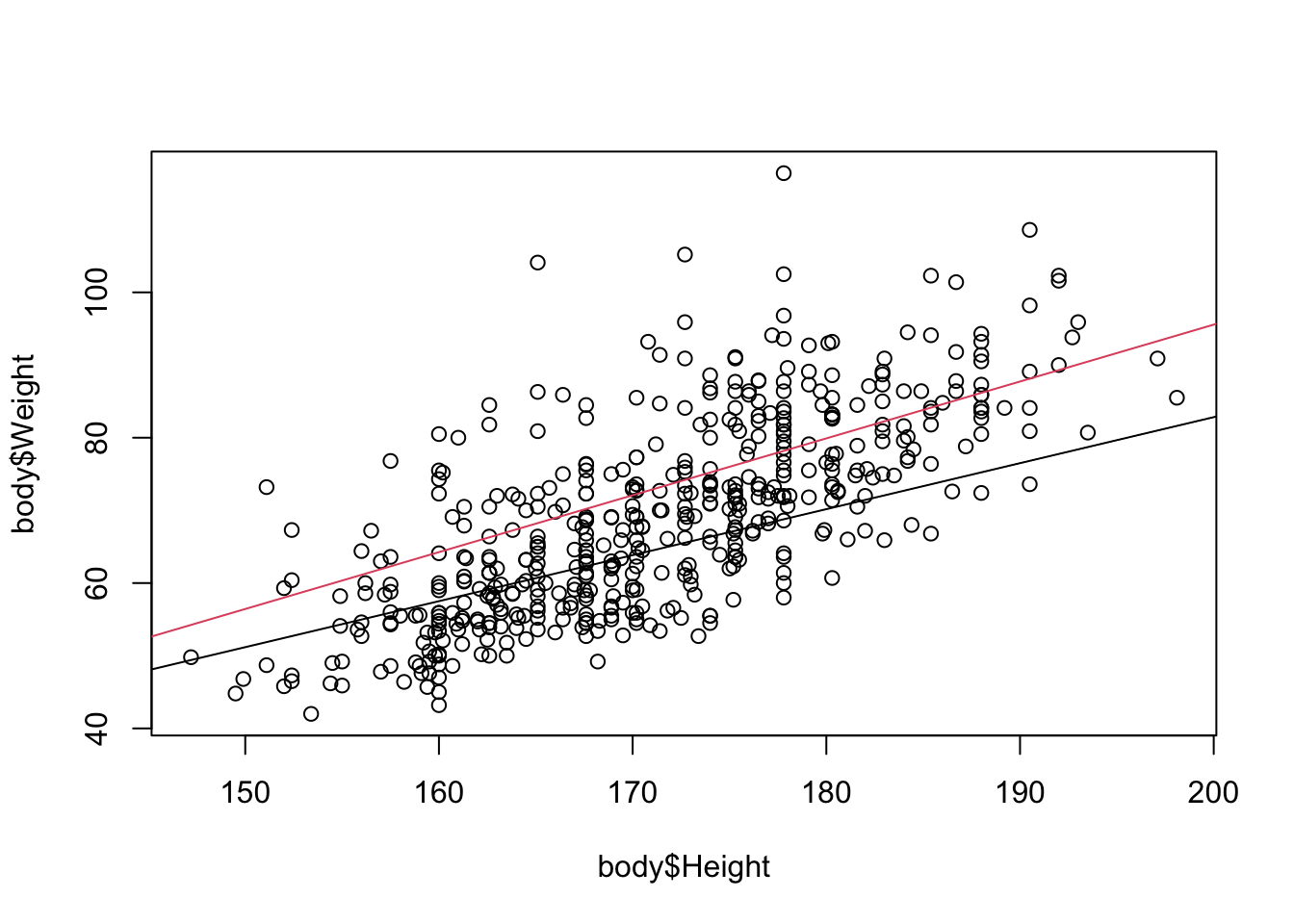
R adjusted set.seed() and other random number generator defaults starting in R version 3.6.0. As such, please ensure the R installation you have is >= 3.6.0. — you can see what version is installed in the header at startup, or type the following into your console: R.Version()$version.string).↩︎
this post does a good job of explaining it, but it is heavier on the theory I expect you to follow for this course↩︎
If you are interested in more than what is presented in this lab, you can always access the help file using ?loess and explored the References for this function.↩︎
As noted in lecture, most of the results follow the general rule that testing MSE’s will be larger than training MSE’s, though by chance this is not currently holding for the linear model.↩︎