A refresher on R and introduction to Quarto documents
Author
Dr. Irene Vrbik
Introduction
This lab session focused on refreshing your R skills and guiding you through the creation of reproducible documents using Quarto. Reproducibility is a cornerstone of modern data analysis, ensuring that results can be consistently reproduced and verified by others. In this lab, we will revisit key R programming concepts and learn how to leverage Quarto for creating dynamic, shareable reports that integrate code, data, and narrative.
Lab Objectives:
By the end of this lab you will be able to:
Execute fundamental R operations, including data manipulation, visualization, and basic statistical analysis.
Describe what Quarto is and explain its importance in reproducible research.
Create a Quarto document that integrates narrative, code, and results, following a step-by-step guide to achieve a fully functional and reproducible report in HTML format. Specifically, you will:
Use basic Markdown for formatting text.
Navigate and utilize the visual editor in RStudio.
Embed R code into Quarto documents using code chunks.
Apply helpful chunk options for both input and output.
Explore different output formats including HTML, PDF, and Word.
Quarto (https://quarto.org/) an open-source publishing system and the next-generation version of R Markdown. Quarto allows you to create dynamic content using multiple programming languages (including Python, Julia, and Observable) across various formats (such as articles, presentations, dashboards, websites, blogs, and books). In this course, we will show you how to use RStudio with Quarto specifically to create assignment documents that integrate R.
Why
Quarto will serve as a great tool for creating well-structured, professional-looking reports that are easy to read and follow. Furthermore, quarto promotes reproducibility by combining narrative, code, and results in one document, ensuring that analyses are transparent and can be replicated by others; a crucial component in scientific research and data analysis. Quarto documents can be easily shared with others, making it simple to collaborate on group projects or receive feedback from peers or instructors. While we won’t cover this aspect in this course, it is worth noting that Quarto works well with version control systems like Git, allowing students to track changes, collaborate on code, and maintain a history of their work.
Now you should have everything you need to get started.
Getting Started
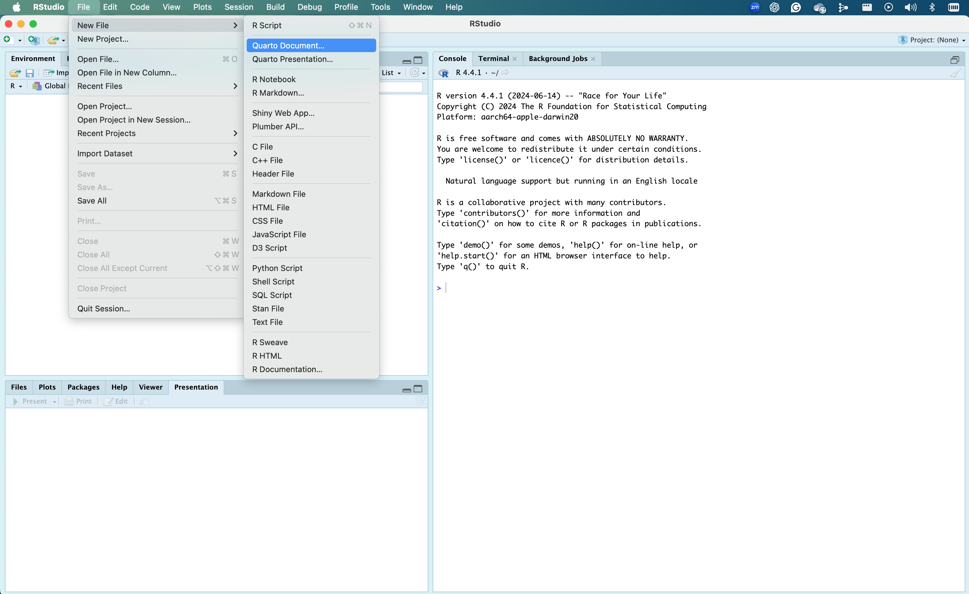
Open R studio and create a new quarto document by navigating to: File > New File > R Script
How to create a new Quarto document. This screenshot was taken in RStudio on a Mac. Depending on your RStudio settings and your computer, your interface might look slightly different.
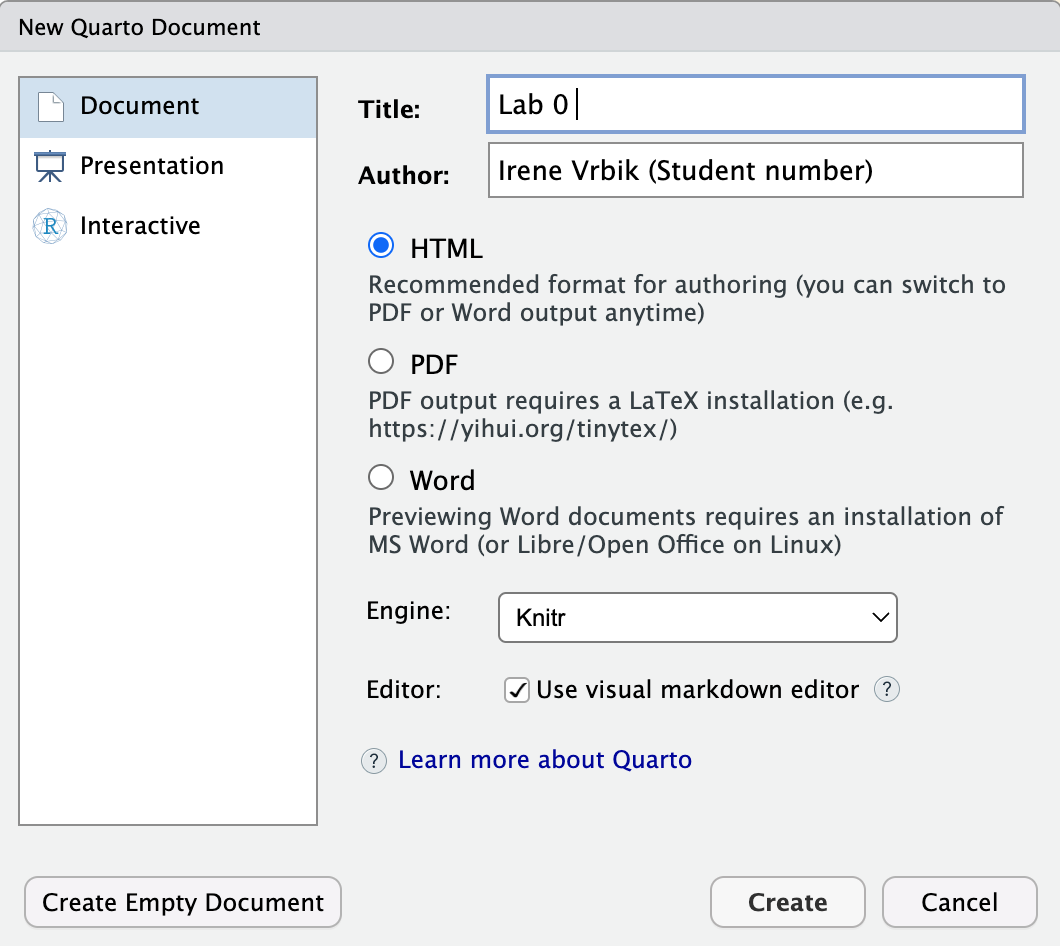
Give your document a meaningrul title, and get in the habbit of using your First and Last name along with your student number in the Author field. Leave the default settings of HTML output and visual editior and press Create.
Recommended Workflow
Render on Save
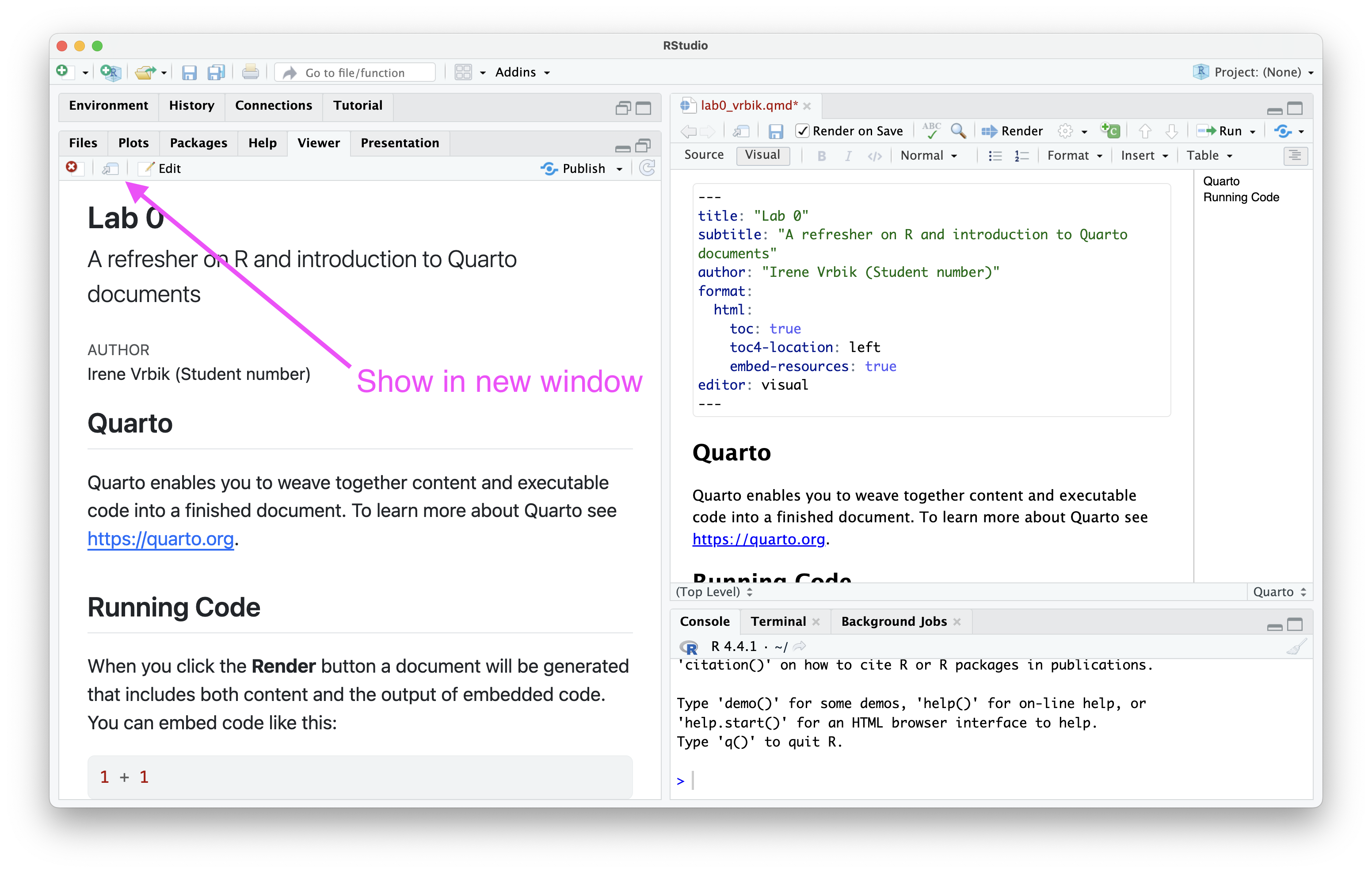
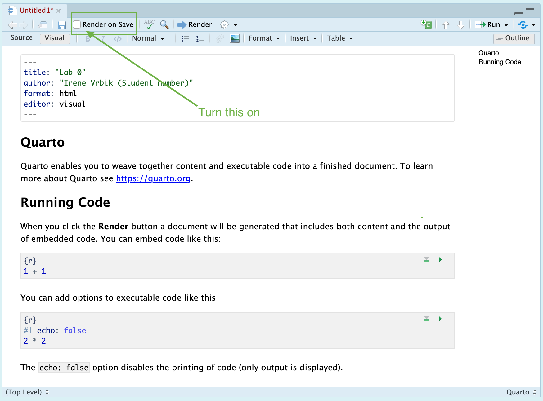
At this point, you should get a document that looks something like the following.
A default qmd file. I recommend getting the habit of enabling the “Render on Save” option.
I recommend that you turn on the “Render to Save” option. When enabled, each time you save the document (e.g. by pressing Ctrl + S or Cmd + S), RStudio will automatically render the document to the specified format. This is particularly useful for continuously previewing changes as you edit your document, allowing for an efficient and iterative writing and editing process.
Render as you go and before submission
Be sure to render your document your document frequently. Always render before submitting or sharing your document to ensure that it is complete, accurate, and free of errors.
Be sure to render your document frequently! For example, I tend to render my document every time I finish a paragraph or write a new code chunk at minimum. If you wait to render your document until the end of your report, you may encounter cryptic error messages that are difficult to troubleshoot. By rendering as you go, it becomes easier to identify and resolve the source of any rendering issues as they arise. Finally, always render before submitting or sharing your document to ensure that it is complete, accurate, and free of errors.
Preview in Panel
By default, your rendered HTML will appear in a separate window. I find it more convenient to view the rendered document side-by-side my .qmd file directly in my RStudio. To enable this, simply change the default settings to “Preview in Viewer Pane”
Now, when you render your .qmd file, a preview your document will appear direct within the viewer pane of RStudio. This feature provides a live preview of how your Quarto document will look once rendered, enabling you to see the HTML output without needing to open it in a separate browser or external viewer.
Setting up your folder system
Before you save your document and start editing, I recommend that you set a dedicated folder in your Documents where all your Data 311 files will be housed. Save your newly created quarto document somewhere within that folder. For instance, you might choose to set up your folder system as follows:
For assignments I will be requiring that you name your document assignment<#>_<student number>. To keep with that nomenclature I suggest that you name this document assignment0_xxxxx.qmd (where xxxxx is replaced by your student number).
R Projects (optional)
Note
If you are just getting started with Quarto and/or you don’t have previous experience with markdown publishing systems, you can skip learning about projects for now. Once you are comfortable with the basics, come back to this section to learn more.
Once you are done Setting up your folder system, I recommend you set up an RStudio Project. An R project creates a dedicated workspace for you to keeps all related files (e.g. scripts, data, documents, and outputs) together in one location. When you are ready to return to the course material you can open the R Project (having extension .Rproj) and RStudio will automatically pick up where you left off. In addition, this setup makes it easy to switch between different tasks (if, for example, you have another R Project for another course) and integrates easily with Git and GitHub (which will not be covered in this course).
To start a new R Project
In RStudio, go to the top menu and select File > New Project.
Choose the Project Type:
Select New Directory if you’re starting fresh.
Choose Existing Directory
Browse to the location of your Data 311 folder on your computer, select and click Open.
Create the Project:
Click Create Project.
RStudio will now create a project file (Data 311.Rproj) inside the Data 311 folder.
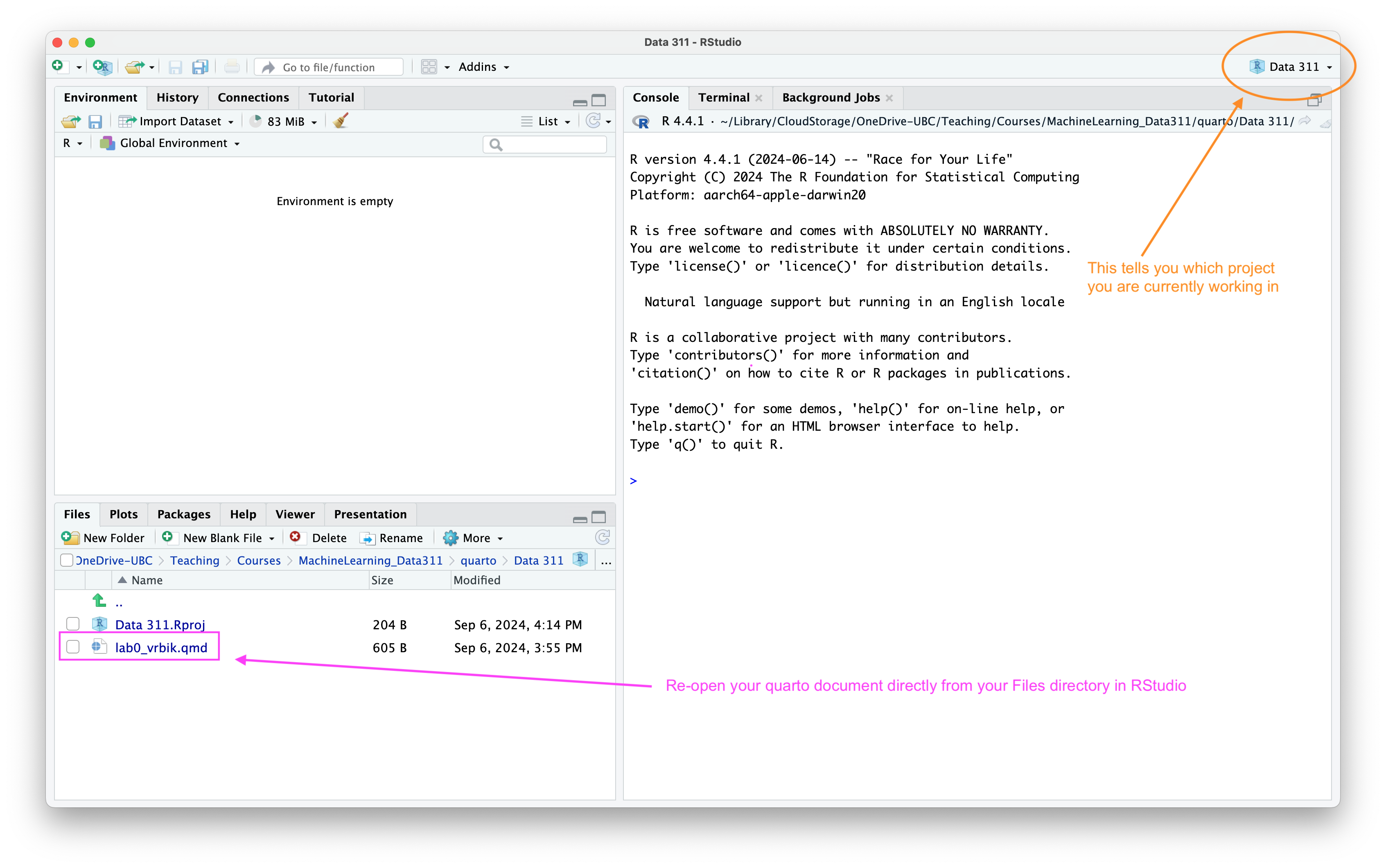
Your project will now open up and you can reopen your lab document directly from the Files panel from R studio.
An RStudio Project. Notice how the name of the project will be indicated in the top right-hand corner, and the Files panel will now match whichever directory your .Rproj file was created.
qmd Overview
This section will cover the various elements commonly found in a typical Quarto document.
YAML
At the top of you document you will see a YAML header demarcated by three dashes (---) on either end. This is is where you specify the metadata and key settings that control how your document is rendered and formatted.
You can customize your YAML by adding various options. For example, you can include a subtitle and enable a table of contents with the following changes to your YAML (please note that nested indentation when setting HTML options):
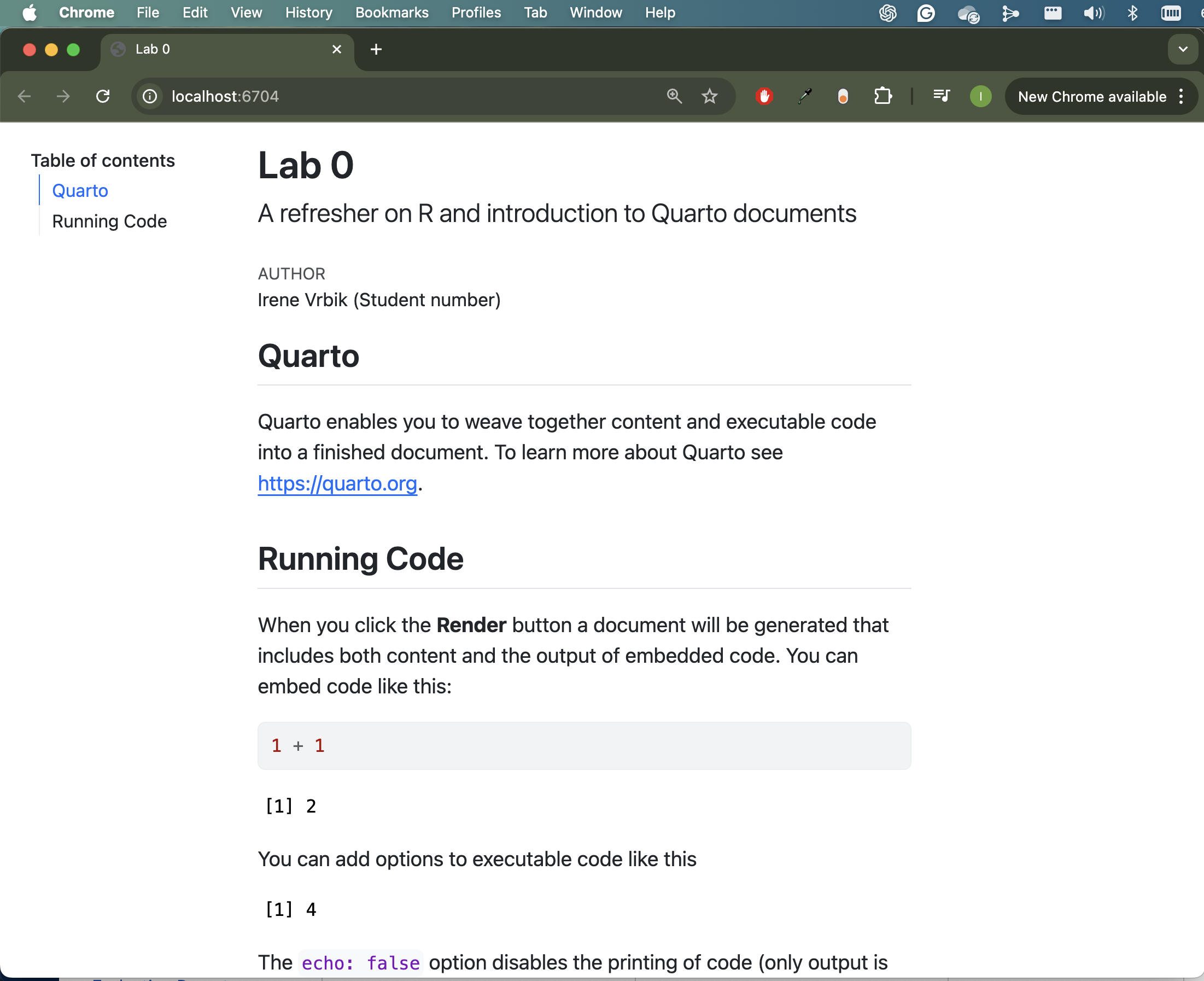
Viewing HTML in external brower
Depending on how big your screen is you might not be able to see your table of contents. If you press the “Show in new window button” () the HTML document will open into your default browser and you should be able to view it on the right-hand-side2.
---
title: "Lab 0"
subtitle: "A refresher on R and introduction to Quarto documents"
author: "Irene Vrbik (Student number)"
format:
  html:
    toc: true
    embed-resources: true
editor: visual
---
I’ve also set the HTML option embed-resources: true. This option embeds external resources such as images, CSS, JavaScript, and fonts directly into the self-contained HTML file instead of linking to these resources as separate files. Since I will only be requesting the HTML file for assignment submissions, this setting is essential; without it, resources like images will not be visible in your submission because they would remain as external links. By embedding these resources, you ensure that everything needed to display your document correctly is included within the HTML file, allowing me to see your images and any other embedded content without additional files.
Embedding Resources
Be sure to include embed-resources: true in your assignment Quarto documents. This enables the embedding of external resources (like images) directly into the rendered HTML document.
Code Chunks
R code chunks identified with {r} with (optional) chunk options, in YAML style, identified by #| at the beginning of the line.
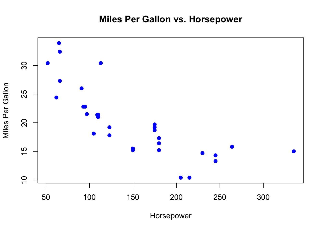
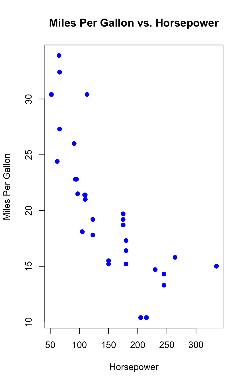
```{r}#| label: fig-code-chunk-example#| fig-cap: "Scatter plot of Miles Per Gallon vs. Horsepower"# Basic scatter plotplot(mtcars$hp, mtcars$mpg, main = "Miles Per Gallon vs. Horsepower", xlab = "Horsepower", ylab = "Miles Per Gallon", pch = 19, # Solid circle point type col = "blue") # Set color of points```
Figure 1: Scatter plot of Miles Per Gallon vs. Horsepower
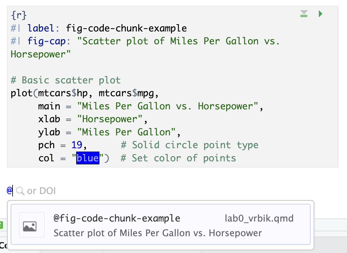
Cross Referencing Figures
Pro tip: Quarto enables you to create cross-references3 to figures, tables, equations, sections, code listings, theorems, proofs, and more.
To create this cross-reference: Figure 1 I simply need tlabel the code chunk that generates the image with a reserved prefix, fig-xxx, where xxx is replaced by a meaningful label (avoid using underscores). If you type @ in your .qmd source file Rstudio’s autocomplete or code completion feature will attemp to assist you by suggesting possible completions. In this case, since I labeled my code chunk fig-code-chunk-example I would cross-reference it using @fig-code-chunk-example.
When RStudio provides a list of possible options as you type, it’s called autocomplete or code completion. This feature is designed to assist you by suggesting possible completions based on what you’ve started typing, which can include function names, variable names, code chunk labels, or references, like in your case with cross-references.
Evaluate code cells. If false just echos the code into output (this is handy for code chunks that take a long time to execute).
code-fold
Collapse code into an HTML <details> tag so the user can display it on-demand.
true: collapse code
false (default): do not collapse code
show: use the <details> tag, but show the expanded code initially.
code-summary
Summary text to use for code blocks collapsed using code-fold
cache
Whether to cache a code chunk. When evaluating code chunks for the second time, the cached chunks are skipped (unless they have been modified), but the objects created in these chunks are loaded from previously saved databases (.rdb and .rdx files), and these files are saved when a chunk is evaluated for the first time, or when cached files are not found (e.g., you may have removed them by hand). Note that the filename consists of the chunk label with an MD5 digest of the R code and chunk options of the code chunk, which means any changes in the chunk will produce a different MD5 digest, and hence invalidate the cache.
warning
Include warnings in rendered output.
error
Include errors in the output (note that this implies that errors executing code will not halt processing of the document).
label
Unique4 label for code cell. Used when other code needs to refer to the cell (e.g. for cross references fig-samples or tbl-summary)
fig-width:
width for figures; the default width for figures is 7 inches.
fig-height
height for figures; the default height for figures is 5 inches.
fig-cap
Figure caption
out-width
Width of the plot in the output document, which can be different from its physical fig-width, i.e., plots can be scaled in the output document. When used without a unit, the unit is assumed to be pixels. However, any of the following unit identifiers can be used: px, cm, mm, in, inch and %, for example, 3in, 8cm, 300px or 50%.
out-height
Height of the plot in the output document, which can be different from its physical fig-height, i.e., plots can be scaled in the output document. Depending on the output format, this option can take special values. For example, for LaTeX output, it can be 3in, or 8cm; for HTML, it can be 300px.
For example, see Figure 2 for the rendered output as produced by the following:
```{r}#| echo: false#| label: fig-chunk-opt-example#| fig-cap: "Notice how in this figure 1. you cannot see the souce code 2. we have resized the outputed image to 4.5 x 7 inches (rather than the default 7 x 5)."#| fig-width: 4.5#| fig-height: 7# Basic scatter plotplot(mtcars$hp, mtcars$mpg, main = "Miles Per Gallon vs. Horsepower", xlab = "Horsepower", ylab = "Miles Per Gallon", pch = 19, # Solid circle point type col = "blue") # Set color of points```
Figure 2: Notice how in this figure 1. you cannot see the souce code 2. we have resized the outputed image to 4.5 x 7 inches (rather than the default 7 x 5).
Question: What do you suppose will happen if you change the default out-width?
Click to view answer
out-width controls how the figure is displayed within the document relative to the surrounding text or page layout; typically specified as a percentage (%), pixels (px), or other CSS units (like cm, in). For instance, “50%”` means that the figure will be rescaled to occupy the 50% of the full width of the text block or container in which it is displayed.
out-width: "50%" means that the figure or output will occupy the 50% of the full width of the text block or container in which it is displayed.
Inline R code
In Quarto, you can include inline R code within your document to dynamically insert the results of R calculations directly into your text. This is particularly useful for including calculated values, summaries, or other outputs directly in the narrative of your document. For insance you could write something like:
The mean of the numbers 11, 20, and 40 is `r mean(c(11, 20, 40))`.
which renders to:
The mean of the numbers 11, 22, and 40 is 23.6666667. If you wanted to format this to control the number of digits to the right of the decimal place use the format() function with nsmall set to the desired number.
The mean of the numbers 11, 20, and 40 is `r format(mean(c(11, 20, 40)), nsmall=2)`.
which renders to:
The mean of the numbers 11, 20, and 40 is 23.66667.
This feature is handy also to call variables you have defined in previous code. For example I can define:
x <-c(11, 20, 40)xbar <-mean(x)
and use:
The mean of `r x` is `r xbar`.
which renders to:
The mean of 11, 20, 40 is 23.6666667.
Markdown
Markdown is a lightweight markup language that allows you to format text easily using plain text syntax. It’s commonly used in Quarto documents for creating headings, lists, links, tables, code blocks, and more. While Markdown is powerful and easy to learn, Quarto also offers a Visual Editor that simplifies document creation without needing to memorize Markdown syntax. The Visual Editor provides a WYSIWYG (What You See Is What You Get) interface that allows you to format text using toolbar buttons, similar to word processors like Microsoft Word or Google Docs. By using the Visual Editor, you can quickly format your document without delving into the underlying Markdown code, allowing you to focus more on content and less on syntax.
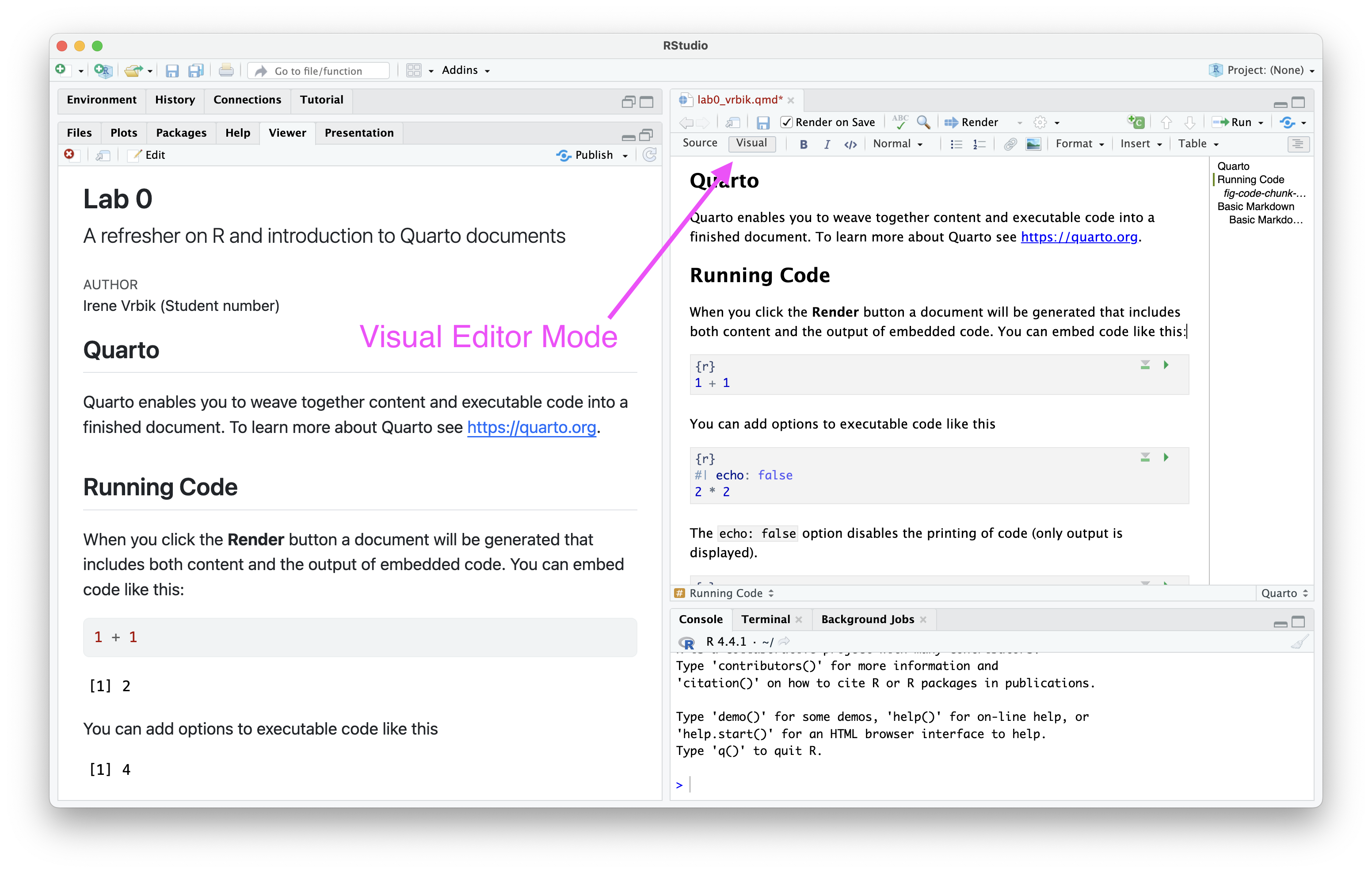
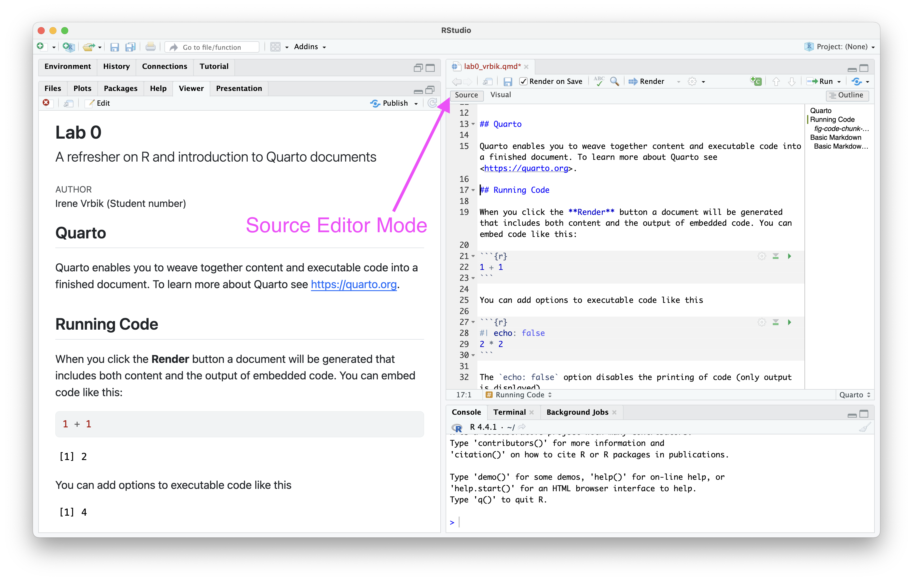
That said, understanding basic Markdown can greatly enhance the readability and organization of your documents. To see whats happening in markdown, you can switch to Source editor; see Figure 3 how to easily toggle back to Visual editor.
(a) Visual Editor Mode
(b) Source Editor Mode
Figure 3: These buttons will help you toggle between Visual editor mode (which is typically the default and in RStudio) and the Source Editor. The Source Editor mode allows you to write and edit your document directly using Markdown, code, and YAML. The Visual Editor mode provides a WYSIWYG (What You See Is What You Get) interface, similar to traditional word processors like Microsoft Word or Google Docs.
Basic Markdown Syntax
Here are some of the most commonly used Markdown elements:
Headings: Create headings by using the # symbol followed by a space. The number of # symbols indicates the heading level.
Bold and Italics: Use asterisks or underscores to emphasize text.
**Bold Text** or __Bold Text__
*Italic Text* or _Italic Text_
Lists:
Unordered Lists: Use *, -, or + followed by a space.
- item 1
- item 2
  - sub-item
Ordered Lists: Use numbers followed by a period.
1. first item
2. second item
3. third item
Links: Create links using square brackets followed by parentheses.
[Quarto Website](https://quarto.org)
Images: Similar to links but prefixed with an exclamation mark.

R Basics for Data Wrangling
Data wrangling, also known as data cleaning or data manipulation, is an essential skill in data analysis that involves transforming and preparing raw data into a usable format. In R, several functions and packages facilitate efficient data wrangling. Here, we’ll cover some basic techniques using base R and the dplyr package from the tidyverse, which provides a consistent and user-friendly syntax for data manipulation.
Loading Data
Before you can wrangle data, you need to load it into R. Common functions for loading data include:
Reading CSV files:
data <-read.csv("path/to/your/data.csv")
Tip 1: Relative paths
When working with data files or images in R, it’s best practice to use relative paths instead of absolute paths. A relative path specifies the location of a file relative to your project’s root directory, rather than the full path from your computer’s root directory. This approach makes your code more portable, shareable, and easier to manage within a project.
When loading data or saving outputs, use paths relative to your project directory. For example, after Setting up your folder system in my R projects, if your data file is stored in a data/ subfolder, I would use the following relative path:
data <-read.csv("data/mydata.csv")
rather than the following absolute path:
data <-read.csv("C:/Users/YourName/Documents/Data_311/data/mydata.csv")
Loading packages
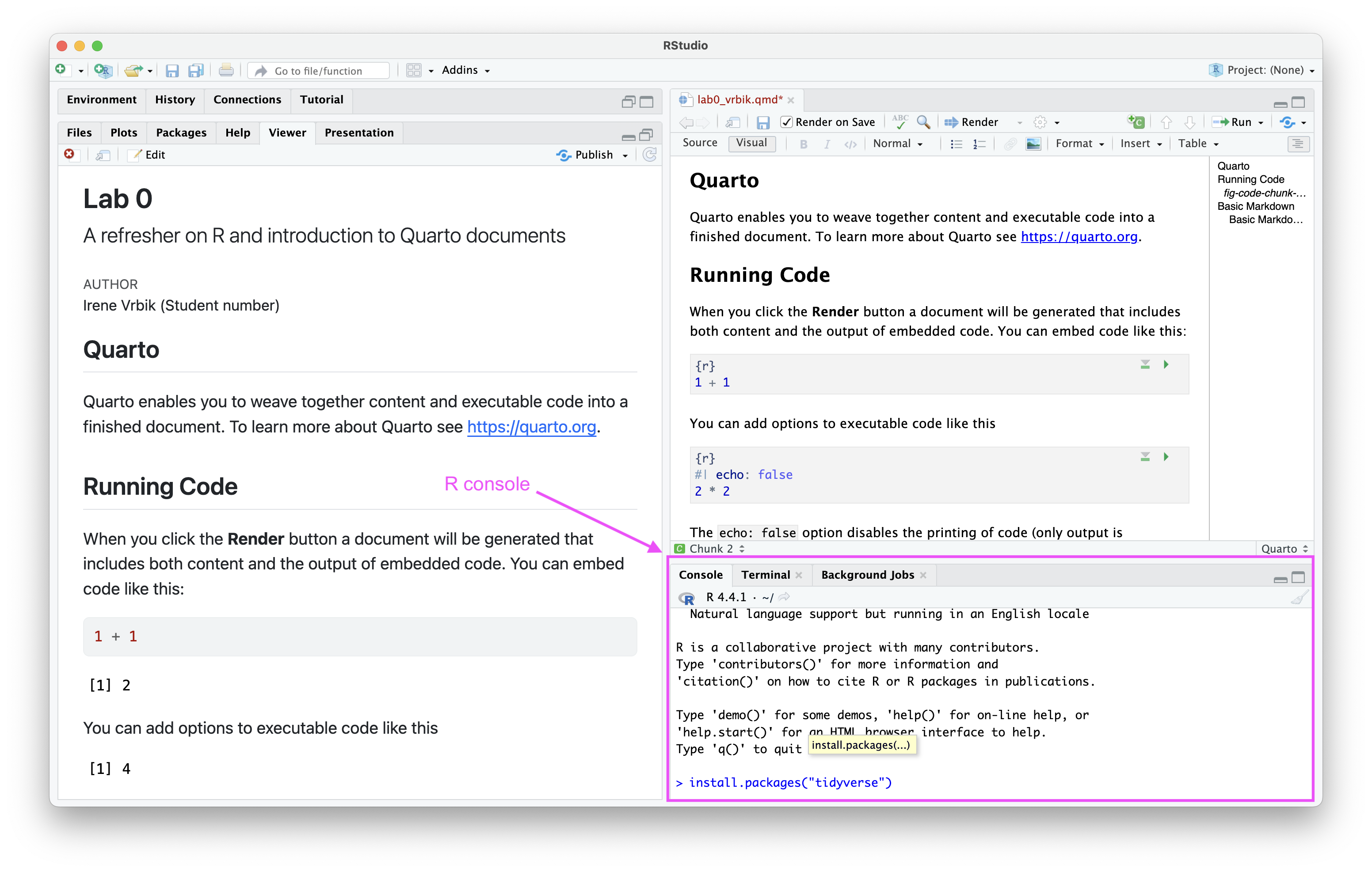
We will often make use of various packages in R. To download package from CRAN, open your R console or RStudio and install the required packages manually using:
install.packages("xxx")
where xxx is replaced by the package name (case sensitive). For example, a very common package used in Data Science is the tidyverse package.
A screenshot showing how you can download a package in the R console. You should never include `include.packages()` in your qmd script. More generally, you should use the R Console for quick, exploratory analyses or trying out code snippets that you don’t want to save to your document (e.g. debugging or testing).
Download this package (if you don’t have it already) using
install.packages("tidyverse")
Installing packages
Never use install.packages() directly within your Quarto (.qmd) script.
Question:Why should you avoid including install.packages() code in a .qmd script.
Click to view answer
Each time the script is rendered or re-run, it will attempt to install the package again, even if it is already installed. This redundancy is unnecessary and can significantly slow down the rendering process. Additionally, if you are not connected to the internet, the script will fail to render because it cannot download the package from CRAN.
After you have downloaded the package (you should do this directly
Viewing and Exploring Data
View the structure of the data:
str(data)
Preview the first few rows:
head(data)
Data Summary and checking for missing values
For numerical data (e.g., integers, doubles), summary(data) displays statistics like the minimum, first quartile, median, mean, third quartile, and maximum. It also shows the number of NA values (missing values) in the column as part of the summary. E.g.
summary(airquality)
     Ozone           Solar.R           Wind             Temp
 Min.   :  1.00   Min.   :  7.0   Min.   : 1.700   Min.   :56.00
 1st Qu.: 18.00   1st Qu.:115.8   1st Qu.: 7.400   1st Qu.:72.00
 Median : 31.50   Median :205.0   Median : 9.700   Median :79.00
 Mean   : 42.13   Mean   :185.9   Mean   : 9.958   Mean   :77.88
 3rd Qu.: 63.25   3rd Qu.:258.8   3rd Qu.:11.500   3rd Qu.:85.00
 Max.   :168.00   Max.   :334.0   Max.   :20.700   Max.   :97.00
 NA's   :37       NA's   :7
     Month            Day
 Min.   :5.000   Min.   : 1.0
 1st Qu.:6.000   1st Qu.: 8.0
 Median :7.000   Median :16.0
 Mean   :6.993   Mean   :15.8
 3rd Qu.:8.000   3rd Qu.:23.0
 Max.   :9.000   Max.   :31.0
Selecting Columns
Use the select() function from the dplyr package (this is included in the tidyverse package) to choose specific columns from a data frame:
library(dplyr) # or library(tidyverse) selected_data <-select(data, column1, column2)
R comments
Note my use of th # symbol in the above code chunk. In R, comments are created using the # symbol. Anything that follows the # on a line is treated as a comment and is ignored by the R interpreter. Comments are crucial for making your code readable, understandable, and maintainable, both for yourself and for others who may work with your code in the future.
If we instead wanted to exclude certain columns we use:
excluded_data <-select(data, -column3)
Filtering Rows
Filtering allows you to subset rows based on conditions using the filter() function:
grouped_summary <- data %>%group_by(column2) %>%summarise(mean_value =mean(column1, na.rm =TRUE))
Note
The following sections may not make sense to you if you didn’t take COSC 304 and/or DATA 101. Don’t worry too much if you do not understand what the following code is doing. We will introduce these concepts as needed throughout the course.
Joining Data
Combining multiple data frames is a common task in data wrangling:
Inner join:
joined_data <-inner_join(data1, data2, by ="common_column")
Left join:
left_joined_data <-left_join(data1, data2, by ="common_column")
Pivoting Data
Reshape data using pivot_longer() and pivot_wider() from the tidyr package:
This marks the end of Lab 0. Pay attention to Canvas to see a release of corresponding Assignment (to be released shortly).
Footnotes
Quarto to also supported by other tools such as VS Codes, Jupyter, Neovim, and Editor. To learn more visit https://quarto.org/docs/get-started/ . Please note that support for this course will be provided exclusively in RStudio.↩︎
If you prefer it on the left-hand side, add the option toc-location: left.↩︎
Cross-referencing involves creating a link or reference to another part of the document. For example, you might refer to “Figure 1” when discussing data visualizations, and clicking on this reference could take the reader directly to that figure.↩︎
you will get an error when you render if you try and reuse a chunk label↩︎

 ) the HTML document will open into your default browser and you should be able to view it on the right-hand-side