Data 311: Machine Learning

Lecture 19: Gaussian Mixture Models

Dr. Irene Vrbik

University of British Columbia Okanagan

Learning Objectives

Today we will be looking at a probabilistic approach to clustering called Gaussian Mixture Models. Aims:

• Understand key components of Gaussian Mixture Models.
• Compare & contrast GMMs to other clustering techniques.
• Grasp the role of probabilistic modeling in clustering.
• Explore the Expectation-Maximization (EM) algorithm.
• Apply GMMs to a practical clustering task.

focused on during my PhD thesis

Clustering

Recall: the goal of clustering¹ (a form of unsupervised learning) is to find groups such that all observations are

• more similar to observations inside their group and
• more dissimilar to observations in other groups.

Cluster analysis is widely adopted by various applications like image processing, neuroscience, economics, network communication, medicine, recommendation systems, customer segmentation, to name a few.

1. or cluster analysis or data segmentation

Old Faithful Data

• Description
• Data frame
• Plot
• Code

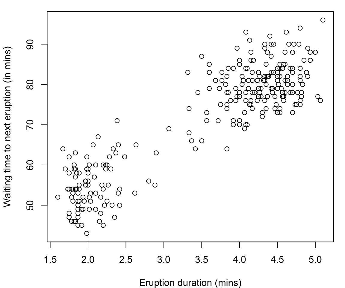
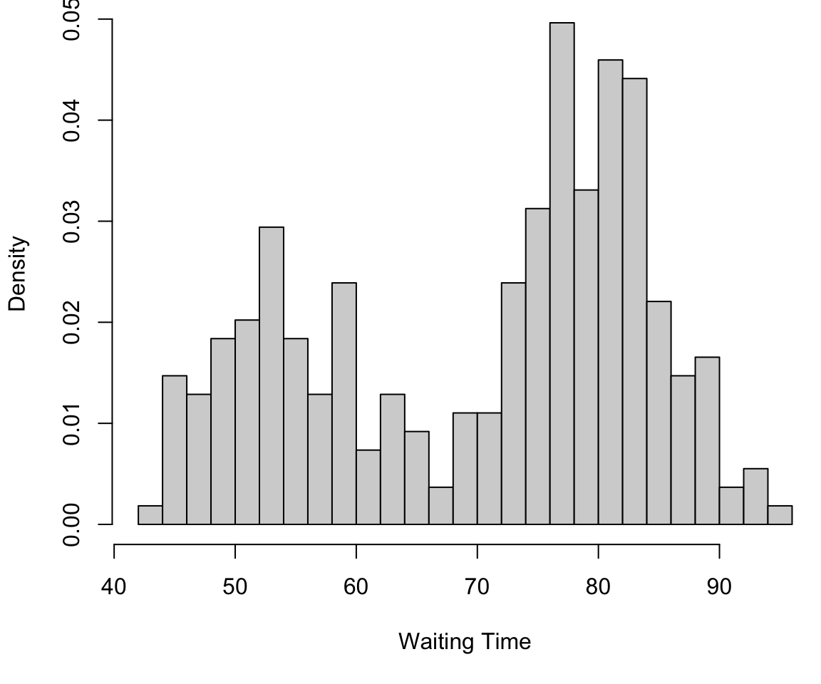
• The faithful dataset in R contains the measurements on time to eruption, and length of eruption time of the Old Faithful geyser in Yellowstone National Park.

• The data frame consists of 272 observations on 2 variables:

  • eruptions Eruption time in mins (numeric)

  • waiting Waiting time to next eruption in mins (numeric)

N.B. to see the help file for any dataset (or function in R) use ?name_of_thing

jump to the iris data set.

Many would argue that there are two clusters:

1. Short eruptions followed shortly thereafter by another eruption
2. Longer eruptions with longer delay before the next eruption

plot(faithful, 
     ylab = "Waiting time to next eruption (in mins)", 
     xlab = "Eruption duration (mins)")

Waiting time between eruptions and the duration of the eruption for the Old Faithful geyser in Yellowstone National Park, Wyoming, USA.

Unsupervised Clustering

• The geyser data falls in the unsupervised clustering problem since there are no predefined labels or outcomes.

• While we can manually identify groupings (i.e. clusters) in lower dimensional space, this is impossible for higher dimensions in which we can no longer visualize our data.

“clustering” –> unsupervised “classification”–> supervised

BUT we get back a “classification” vector when we cluster and we will use “clusters” to describe groups of data points (eg. as we did in iris)

• Unlike the iris data the geyser data set does not have a column of known class labels

Determining Clusters

• Rather than creating the clusters ourselves, we look for automated ways to find these natural groupings.

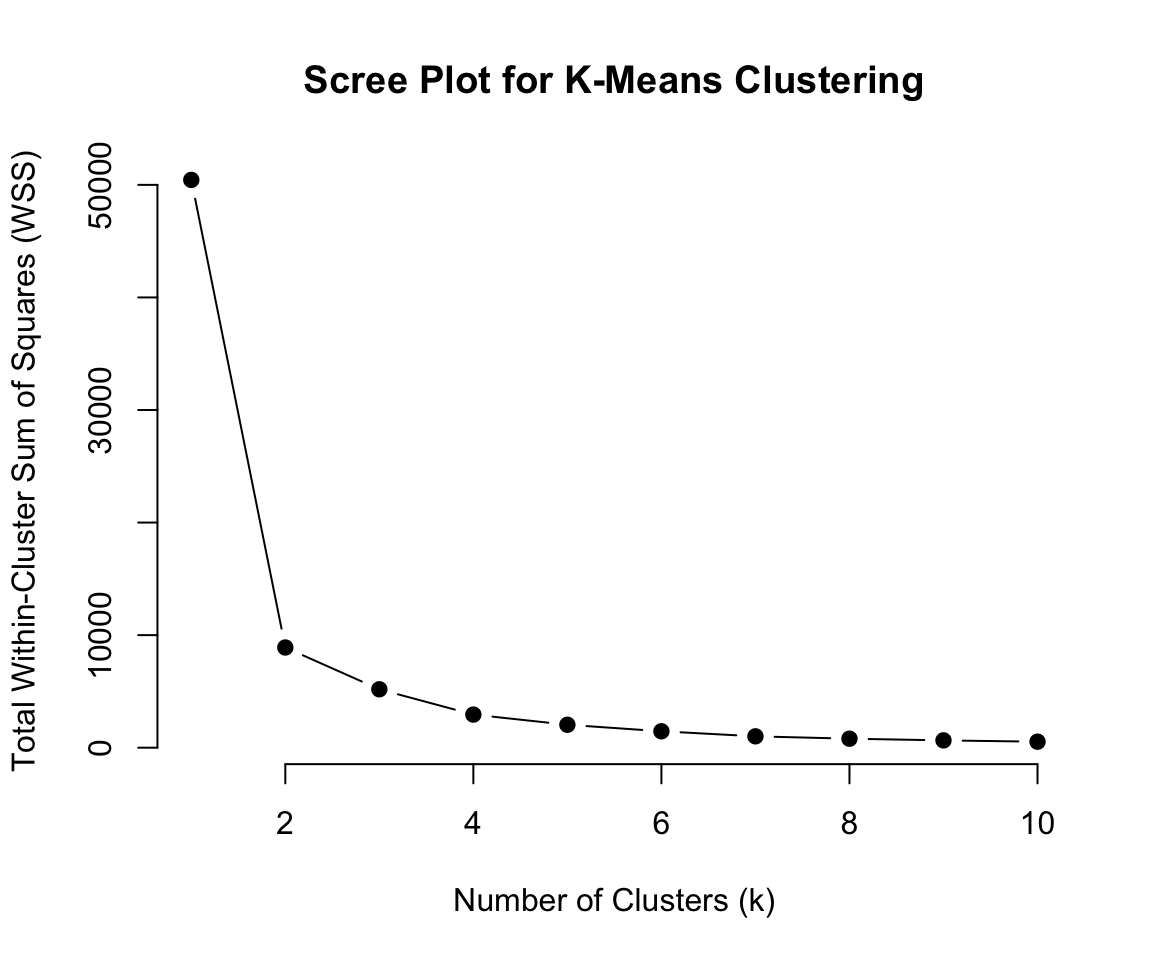
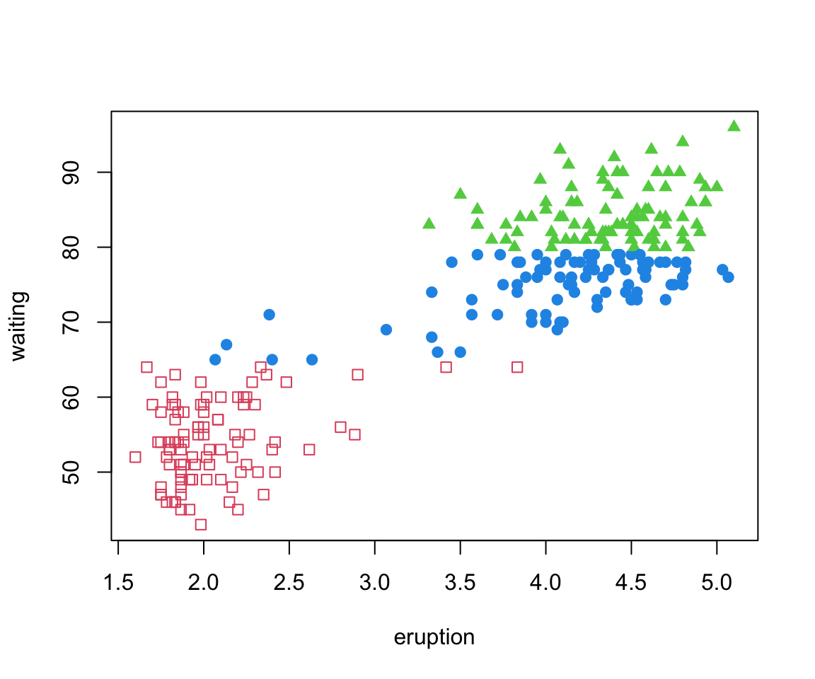
• Previously we saw how k-means and hierarchical clustering can cluster this data

• We used “elbow method” for kmeans and large vertical gaps in the dendrogram to determine the number of clusters.

• Another option could be running Mclust* to obtain a optimal* partition of the data.

these automated techniques often involve some measures of distances

Plot the total within-cluster sum of squares (WSS) or another cost function against the number of clusters ( K).

The “elbow point” is where the rate of decrease sharply changes, indicating diminishing returns for increasing K.

Examine the dendrogram plot and identify a height where clusters are well-separated.

Look for large vertical gaps between successive merges, which suggest natural divisions.

* we’ll return to these points later

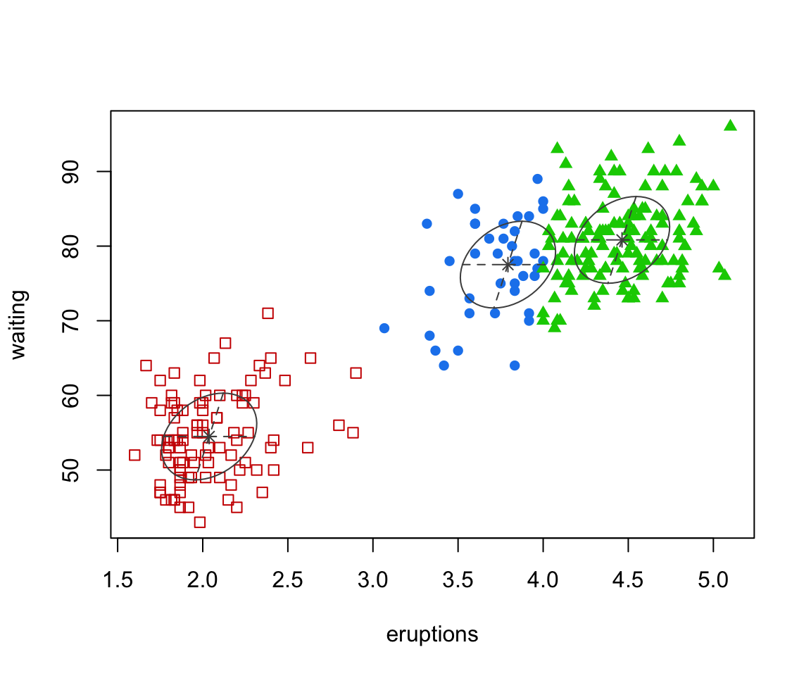
faithful clustered

The points are coloured by group allocation.

Interestingly, mclust determines that there are 3 groups in the data.

But how did mclust determine that 3 clusters was optimal?

Note the difference in capitalization (M for function m for package)

Recall Kmeans

# Load the data
library(MASS)

# Define a function to calculate total within-cluster sum of squares (WSS)
wss <- function(data, k) {
  kmeans(data, centers = k, nstart = 25)$tot.withinss
}

# Compute WSS for k = 1 to 10 clusters
set.seed(42)  # For reproducibility
k_values <- 1:10
wss_values <- sapply(k_values, wss, data = faithful)

# Plot the scree plot
plot(k_values, wss_values, type = "b", pch = 19, frame = FALSE,
     xlab = "Number of Clusters (k)",
     ylab = "Total Within-Cluster Sum of Squares (WSS)",
     main = "Scree Plot for K-Means Clustering")

kout = kmeans(faithful, centers = 3, iter.max = 10, nstart = 25)
plot(faithful, xlab = "eruption", col = kout$cluster+1, pch = c(0,17,19)[kout$cluster])

Recall Kmeans

• Partitions data into \(k\) clusters by minimizing within-cluster variance.
• Assumes spherical clusters and hard assignments.

Limitations:

• Assumes clusters are similar in size and shape.
• Cannot model overlapping clusters.

GMM addresses these limitations with a probabilistic approach.

From k-Means to GMM

Similarities:

• Both partition data into \(k\) clusters.

• Both require the number of clusters \(k\) to be specified in advance.

Kmeans

• centroid-based clustering algorithms

• “hard”¹ clustering

• assumes spherical, equal-sized clusters

GMM

• Distribution-based clustering

• soft² clustering

• supports ellipsoidal clusters and varying sizes

1. Each data point is exclusively assigned to a single cluster.

2. Each data point is assigned a probability or degree of membership for every cluster.

Mixture Models

Resources

[MP] Mixture Model-Based Classification by Paul D. McNicholas

[FS] Finite Mixture and Markov Switching Models by Fruhwirth-Schnatter, S. (2006)

[MG] Finite Mixture Models by McLachlan, Geoffrey J; Peel, David/ New York: John Wiley & Sons

[LB] Mixture models: theory, geometry, and applications by Lindsay, Bruce G

Mixture Models

Mixture models are just a convex combination of statistical distributions. In general, for a random vector \(\mathbf{X}\), a mixture distribution is defined by \[f(\mathbf{x}) = \sum_{g=1}^G \pi_g p_g(\mathbf{x} \mid \theta_g)\] where \(G\) is the number of groups¹, \(0 \leq \pi_g \leq 1\) and \(\sum_{g=1}^G \pi_g = 1\) and \(p_g(\mathbf{x} \mid \theta_g)\) are statistical distributions with parameters \(\theta_g\).

You have probably seen many data sets that are mixtures eg. height of people at UBCO (dist for men vs woman)

• \(\mathbf{X}\) is a \(p\)-dimensional random vector with density \(p(\mathbf{x})\)
• \(\mathbf{X}\) takes values in some sample space in \(R^p\)
• We assume that the density \(p(\mathbf{x})\) is defined with respect to an appropriate measure on \(R^p\)

convex combination where all coefficients are non-negative and sum to 1

\(f(x | \Theta)\) or \(f(x ; \Theta)\) notation where \(\Theta = \{\theta_1,...\theta_G, \pi_1, ....,\pi_G\}\)

1. aka clusters or components

Terminology

• The \(\pi_g\) are called mixing proportions and we will write \(\mathbf{\pi} = (\pi_1, \pi_2, \dots, \pi_G)\)

• The \(p_g(\mathbf{x})\) are called component densities

• Since the \(p_g(\mathbf{x})\) are densities, \(f(\mathbf{x})\) describes a density called a \(G\)-component finite mixture density.

Statistical Distributions

• In theory, \(p_g(\mathbf{x} \mid \theta_g)\) could be a different distribution type for each \(g\).

• In practice, however, \(p_g(\mathbf{x} \mid \theta_g)\) is assumed to be the same across groups, but with different \(\theta_g\).

• Most commonly, we assume a a Gaussian mixture model (GMM) where \(p_g(\mathbf{x} \mid \theta_g)\) is assumed to be multivariate Gaussian (aka multivariate Normal), denoted \(\phi(\mathbf{x} | \mu_g, \mathbf{\Sigma}_g)\)

Gaussian Mixture model

Thus \(f(\mathbf{x})\) — sometimes written \(f(\mathbf{x} | \Theta)\) or \(f(\mathbf{x} ; \Theta)\) — is a Gaussian mixture model would have the form: \[\begin{align} f(\mathbf{x} | \Theta) &= \sum_{g=1}^G \pi_g \phi(\mathbf{x} \mid \boldsymbol\mu_g, \mathbf{\Sigma}_g) \\ &= \sum_{g=1}^G \pi_g \frac{|\mathbf{\Sigma}|^{-1/2}}{(2\pi)^{k/2}} \exp \left( - \frac{1}{2} (\mathbf{x} - \boldsymbol{\mu}_g)^{\mathrm {T}} \mathbf{\Sigma}^{-1} (\mathbf{x} - \boldsymbol{\mu}_g) \right) \end{align}\] where \(\phi\) denote the normal distribution, \(\boldsymbol{\mu}_g\) is the mean vector for group \(g\) and \(\mathbf{\Sigma}_g\) is the covariance matrix for group \(g\), and \(\Theta = \{\boldsymbol{\mu}_1, ..., \boldsymbol{\mu}_G, \mathbf{\Sigma}_1, ..., \mathbf{\Sigma}_G, \pi_1, ..., \pi_G\}\)

See

Components of GMM

1. Means (\(\mu_k\)): Cluster centers.

2. Covariances (\(\Sigma_k\)): Shape and spread of clusters.

3. Mixing Coefficients (\(\pi_k\)​): Proportion of data in each cluster.

Distribution Alternatives

Other robust alternatives include:

• Mixtures of Student-\(t\) distributions¹ (heavier tails)

• Mixtures of skewed distributions

  • skew-normal (Lin et al, 2007)
  • skewed-\(t\) Vrbik and McNicholas, 2012

1. (Peel & McLachlan, 2000), (Andrews et. al, 2011)

Finite mixture in 1D

This can be viewed as a mixture of 2 univariate Gaussians….

Finite mixture in 1D

Component 1 (in red) \[f_1 \sim N(\mu = 54.6, \sigma = 5.9)\]

Finite mixture in 1D

Component 2 (in blue) \[f_2 \sim N(\mu = 80.1, \sigma = 5.8)\]

Finite mixture in 1D

And mixture (in black): \[ 0.4 f_1 + 0.6f_2 \]

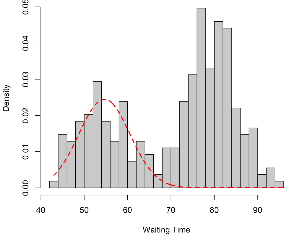
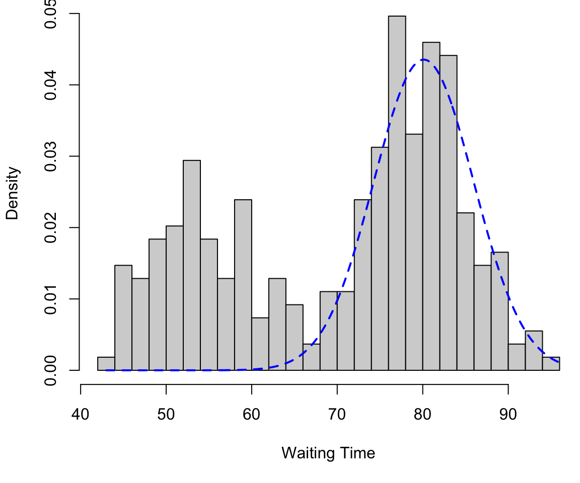
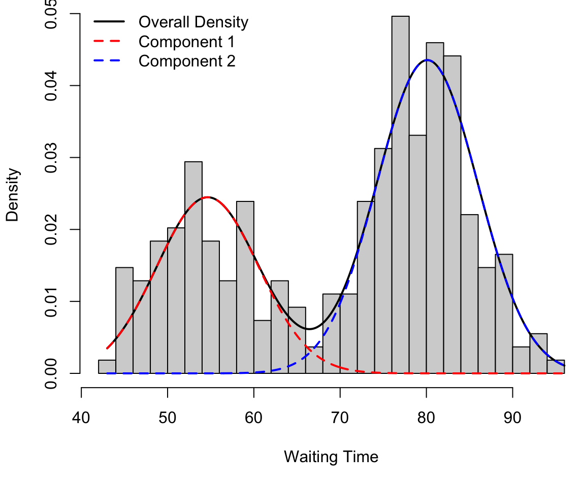
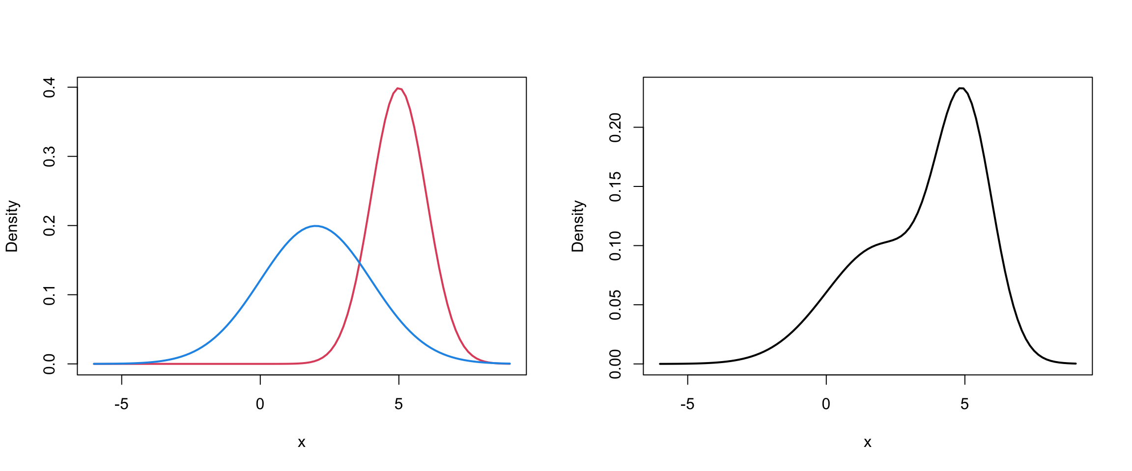
# Load required libraries
library(mclust)

# Load the faithful dataset
data("faithful")
waiting <- faithful$waiting

# Fit a Gaussian Mixture Model with 2 components
set.seed(42)
gmm <- Mclust(waiting, G = 2, modelNames = "V")

# Extract GMM parameters
means <- gmm$parameters$mean
sds <- sqrt(gmm$parameters$variance$sigmasq)
proportions <- gmm$parameters$pro

# Create a sequence for density plotting
x_vals <- seq(min(waiting), max(waiting), length.out = 500)

# Compute individual and overall densities
density1 <- proportions[1] * dnorm(x_vals, mean = means[1], sd = sds[1])
density2 <- proportions[2] * dnorm(x_vals, mean = means[2], sd = sds[2])
overall_density <- density1 + density2

par(mar=c(5,4,0,0) +0.1)
# Plot the histogram and density curves
hist(waiting, freq = FALSE, breaks = 20, main = "",
     xlab = "Waiting Time")
lines(x_vals, overall_density, col = "black", lwd = 2, lty = 1)  # Overall density
lines(x_vals, density1, col = "red", lwd = 2, lty = 2)           # Component 1
lines(x_vals, density2, col = "blue", lwd = 2, lty = 2)          # Component 2
legend("topleft", legend = c("Overall Density", "Component 1", "Component 2"),
       col = c("black", "red", "blue"), lwd = 2, lty = c(1, 2, 2), bty = "n")

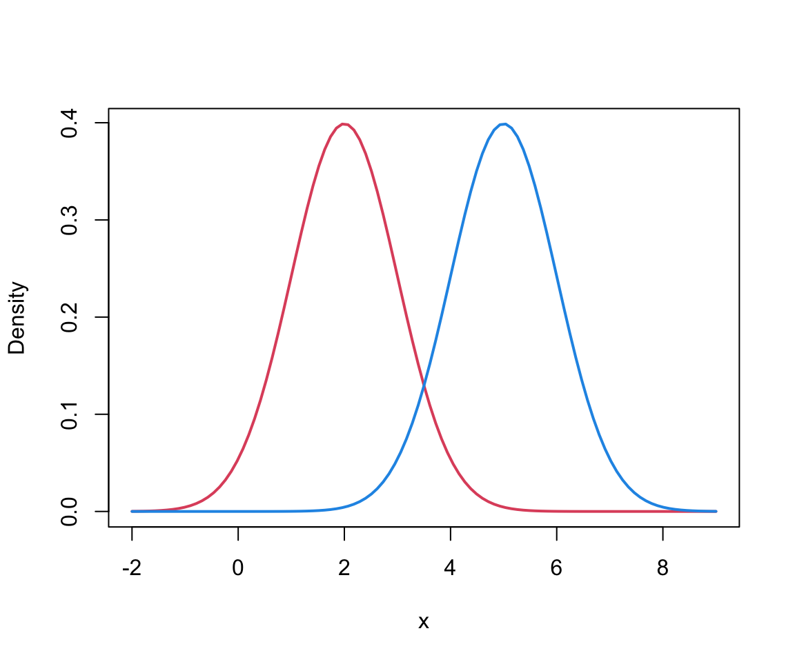
Two Univariate Normals I

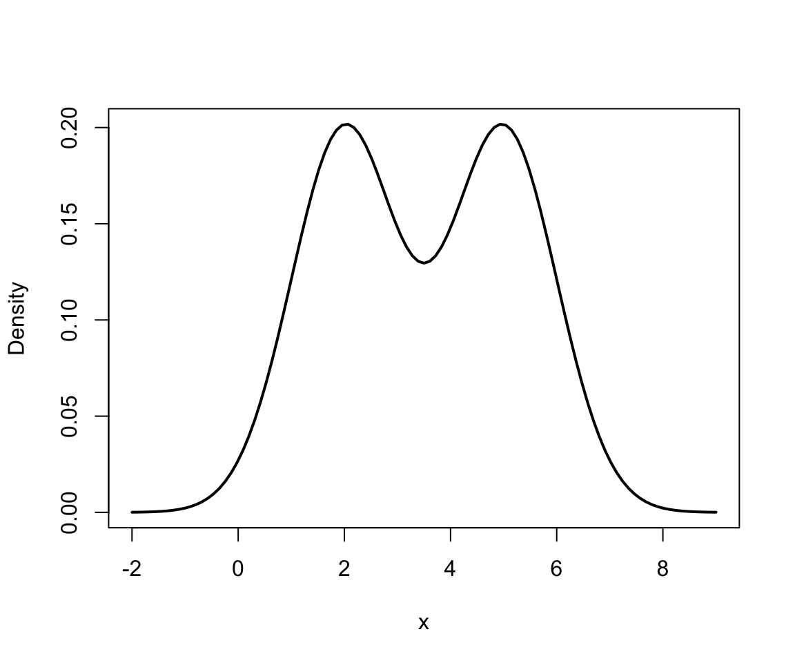
Mixture of 2 univariate Normals II

Mixture of 2 univariate Normals II

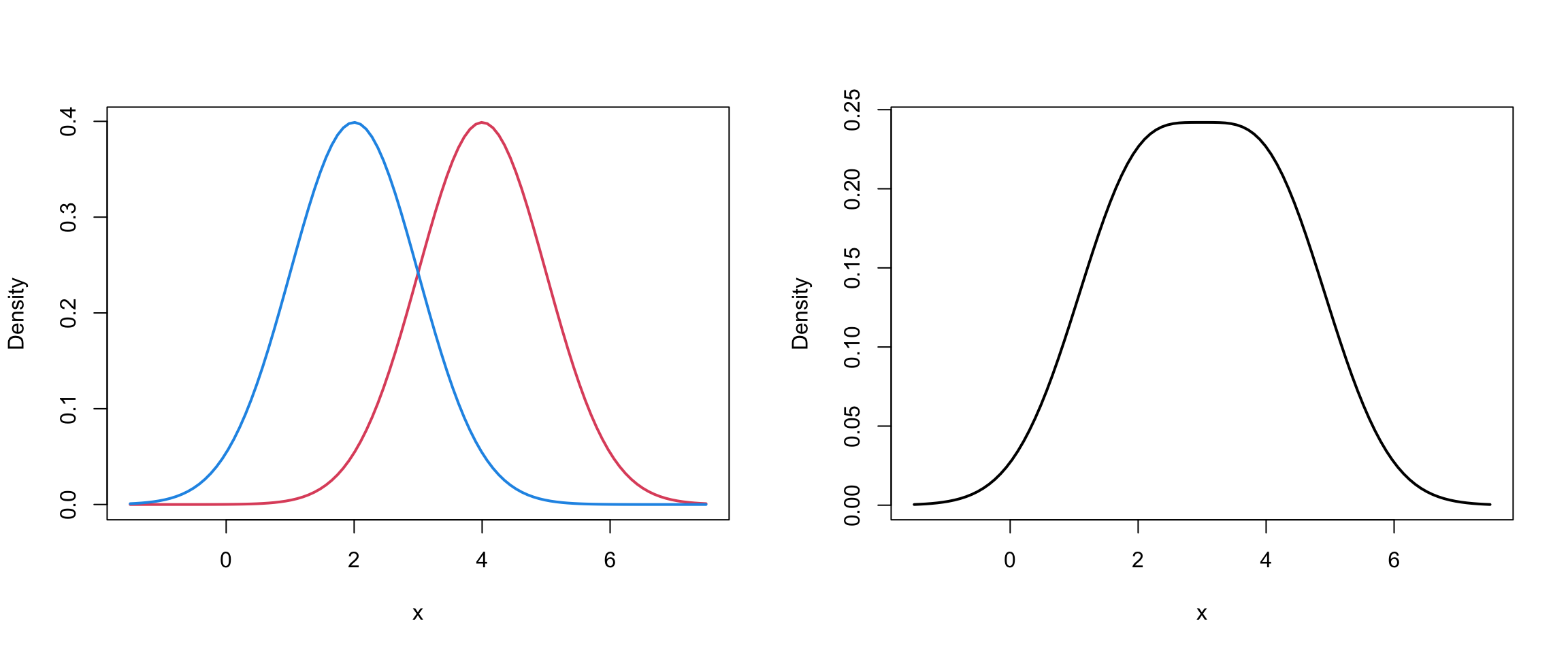
Mixture of 2 univariate Normals III

Identifiability I

• Inference for finite mixture modles is typical in that we want to estimate parameters \(\Theta = \{\theta_1, ... , \theta_G, \pi_1, ...,\pi_G\}\)

• However, this estimation is only meaningful if \(\Theta\) is identifiable.

• In general, a family of densities \(\{ p(\mathbf{x} | \Theta) : \Theta \in \Omega \}\) is identifiable if: \[p(\mathbf{x} | \Theta) = p(\mathbf{x} |\Theta^*) \iff \Theta^* = \Theta\] In the case of mixture models this gets a bit complicated…

Identifiability II

One problem is that component labels may be permuted:

\[\begin{align} p(x | \Theta) &= \pi_1 p(x | \mu_1, \sigma_1^2) + \pi_2 p(x | \mu_2, \sigma_2^2)\\ p(x | \Theta^*) &=\pi_2 p(x | \mu_2, \sigma_2^2) + \pi_1 p(x | \mu_1, \sigma_1^2) \end{align}\]

• The identifiable condition is not satisfied because the component labels can be interchanged yet \(p(x | \Theta) = p(x | \Theta^*)\)

• As [MG] point out, even though this class of mixtures may be identifiable, \(\Theta\) is not.

Futhermore, i can have many more compoents with \(\pi_g\) =0

Identifiability III

• The identifiability issue that arises due to the interchanging of component labels can be handled by imposing appropriate constraints on \(\Theta\)

• For example, the \(\pi_g\) could be constrained so that \(\pi_i \geq \pi_k\) for \(i>k\).

• Also we can avoid empty components by insisting that \(\pi_g > 0\) for all \(g\).

essentially your first group is your smallest group, second group is your second smallest group, … Gth group is your largest

Mixture Models for clustering

• Finite mixture models are ideally suited for clustering

• Clusters correspond to the \(1,...,g,...G\) sub-populations/groups/components in a finite mixtures model.

• So, let’s attempt the to derive the MLE of the Gaussian mixture model …

In one-dimension: \[\begin{align} L(\theta | X_1,\ldots,X_n) &= \prod_{i=1}^n \sum_{g=1}^G \pi_g N(x_i;\mu_g, \sigma_g^2)\\ \ell(\theta) &= \sum_{i=1}^n \log \left( \sum_{k=1}^K \pi_k N(x_i;\mu_k, \sigma_k^2) \right ) \end{align}\] Taking a look at the expression above, we already see a difference between this scenario and the simple setup in the previous section. We see that the summation over the K components “blocks” our log function from being applied to the normal densities. If we were to follow the same steps as above and differentiate with respect to μk and set the expression equal to zero, we would get:

The Likelihood

The likelihood function for this mixture is \[\begin{align} L(\Theta) &= f(\mathbf{x} | \Theta) = \prod_{i=1}^n \left[ \sum_{g=1}^G \pi_g \phi(\mathbf{x} \mid \boldsymbol\mu_g, \mathbf{\Sigma}_g) \right] \end{align}\] and the so-called log-likelihood is: \[\begin{align} \ell(\Theta) &= \log(L(\Theta)) = \sum_{i=1}^N \log\left[ \sum_{g=1}^G \pi_g \phi(\mathbf{x} \mid \boldsymbol\mu_g, \mathbf{\Sigma}_g) \right] \end{align}\]

If you try to differentiate w.r.t. to \(\mu_g\), set =0, and solve, you would find that this has no analytic solution.

the \(\log(\sum)\) is problematic and won’t lead to closed-form solutions

Marginal Likelihood (Sum): When we don’t know the cluster memberships (ZigZ_{ig}Zig​), we sum over all possible assignments (marginalization).

The marginal likelihood of a single data point \(x_i\) is derived by summing over all possible cluster assignments \(Z_{ig}\) \[ \begin{align*} f(x_i \mid \Theta) &= \sum_{g=1}^G p(x_i, Z_{ig} = 1 \mid \Theta) = \sum_{g=1}^G p(Z_{ig} = 1) p(x \mid Z_{ig} = 1)\\ &= \sum_{g=1}^G \pi_g \phi(x_i \mid \mu_g \Sigma_g) \end{align*} \]

Here, \(f(x_i \mid \Theta)\) represents the likelihood of observing \(x_i\)​, irrespective of its cluster membership.

EM algorithm

• Most commonly, we use the expectation-maximization (EM) algorithm, which helps us find parameter estimates with missing data (group memberships are missing).

• More generally, the EM is an iterative algorithm for finding maximum likelihood parameters in statistical models, where the model depends on unobserved latent variables.

• We assume that each observed data point has a corresponding unobserved latent variable specifying the mixture component to which each data point belongs.

In statistics, latent variables (from Latin: present participle of lateo, “lie hidden”) are variables that can only be inferred indirectly through a mathematical model from other observable variables that can be directly observed or measured.

Latent Variable

We introduce a new latent¹ variable that represents the group memberships: \[\begin{equation} Z_{ig} = \begin{cases} 1 & \text{if } \mathbf{x}_i \text{ belongs to group }g \\ 0 & \text{otherwise} \end{cases} \end{equation}\]

We call \(\{X, Z\}\) our “complete” data.

Now that we have that, let’s look at a non-technical summary of the EM algorithm…

Introducing unobserved variables, Zi, to help with computations or derivations is a common trick that is used beyond mixture models.

This trick is sometimes called data augmentation.

The unobserved random variables are sometimes called hidden variables or latent variables.

1. latent is Latin for missing, so you might think of this as missing data

Latent Variable Representation

The joint probability of a data point \(x_i\) and its latent variable \(Z_{ig}\)​ is:

\[ p(x_i, Z_{ig} \mid \Theta) = p(Z_{ig} \mid \Theta) p(x_i \mid Z_{ig}, \Theta) \]

The complete likelihood assumes we know the latent cluster assignments:

\[ \begin{align*} L_c(\Theta) &= \prod_{i=1}^n \prod_{g=1}^G \left[\pi_g \phi(x_i|\mu_g, \sigma_g)\right]^{\hat{z}_{ig}}\\ \ell_c(\Theta) &= \sum_{i=1}^n \sum_{g=1}^G \hat{z}_{ig} \left[ \log (\pi_g) + \log (\phi(x_i|\mu_g, \sigma_g) )\right] \end{align*} \]

Essentially just QDA now.

where \(z_{ig} = 1\) if \(x_i\) belongs to cluster \(g\), and \(z_{ig} = 0\) otherwise.

we assume \(Z_{ig} = \hat z_{ig}\) for each data point

Complete Likelihood (Product): When we treat the cluster memberships (ZigZ_{ig}Zig​) as known, we directly compute the joint likelihood for the observed data and assignments.

This product is simple because only one term (the cluster corresponding to z_{ig} = 1$ contributes to the likelihood

I is an indicator function \(\Pi_g \pi_g \phi_g = \pi_g \phi_g\) for the true group (if we knew Z)

This leads to a simple MLE

We’ll work with univariate normal distribution for simplicity.

EM Pseudocode

1. Start the algorithm with random values for \(\hat z_{ig}\).
2. Mstep: Assuming those \(\hat{z}_{ig}\) are correct, find the maximum likelihood estimates (MLE)
3. Estep: Assuming those parameters are correct, find the expected value of group memberships \[\hat{z}_{ig} = \frac{\pi_g \phi(\mathbf{x} \mid \boldsymbol{\mu}_g, \mathbf{\Sigma}_g) }{\sum_{g=1}^G \pi_g \phi(\mathbf{x} \mid \boldsymbol{\mu}_g, \mathbf{\Sigma}_g)}\]
4. Repeat 2. and 3. until “changes” are minimal.

(there are alternative starting options)

(via MLEs — hence, this is the of EM)

(this is the of EM)

(The log-likelihood of the model is monitored for convergence)

Z –> z to imply no longer R.V

Mstep

For the “M-step”, i.e. maximization step, and given the \(z\)’s calculated in the E-step …

\[ \begin{align*} \mu_g &= \frac{\sum_{i=1}^n z_{ig} x_i}{\sum_{i=1}^n z_{ig}} & \pi_g &= \frac{\sum_{i=1}^n z_{ig}}{n} \end{align*} \] \[ \Sigma_g = \frac{\sum_{i=1}^n z_{ig} (x_i - \mu_g)(x_i - \mu_g)^T}{\sum_{i=1}^N r_{ig}} \]

where \(n\) is the total number of data points.

Fuzzy z’s

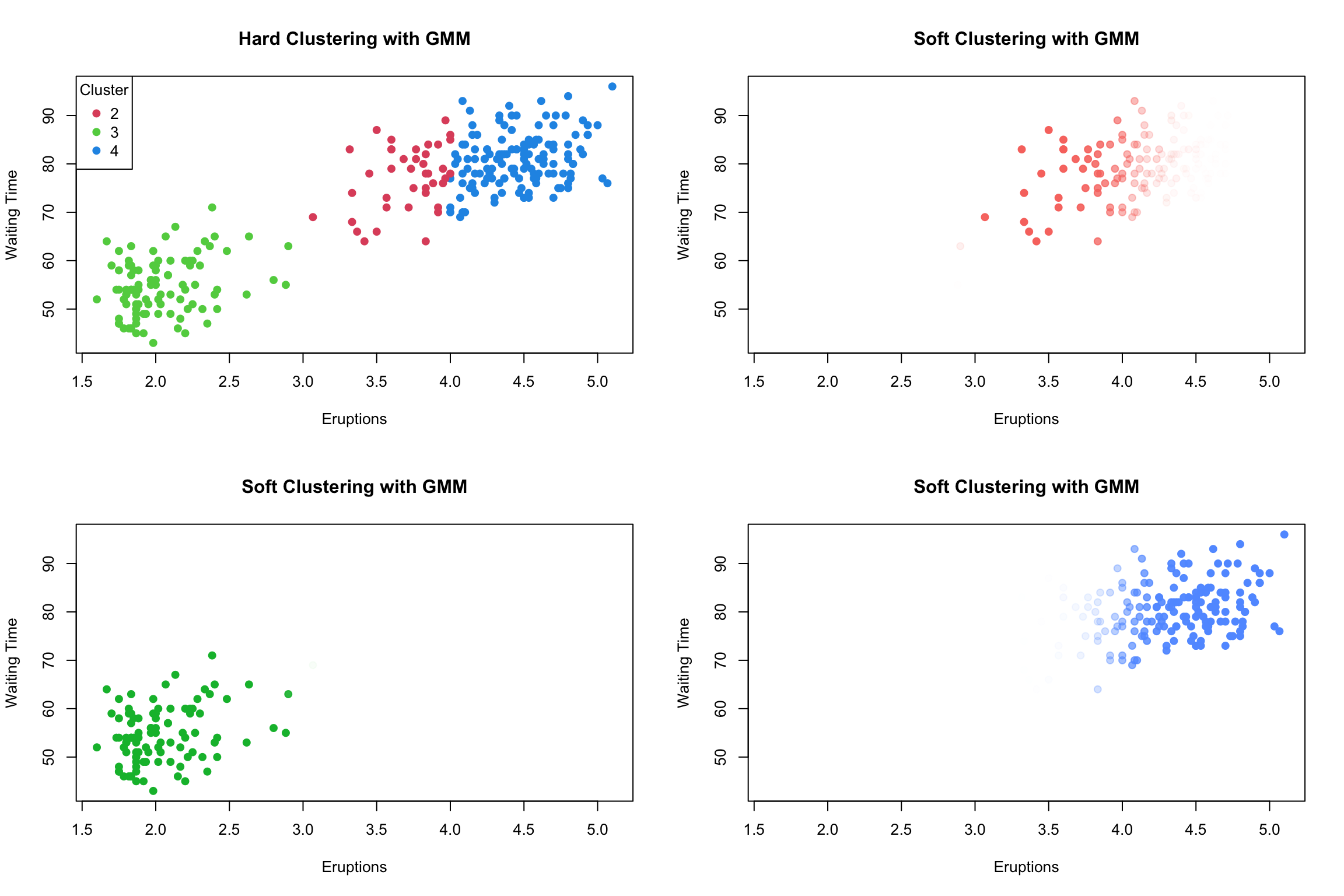
• The resulting \(\hat{z}_{ig}\) are not going to be 0’s and 1’s when the algorithm converges.

• For each observation \(\mathbf{x}_i\) we end up with vector of probabilities (\(\hat{z}_{i1}\),…,\(\hat{z}_{iG}\)) which we denote by \(\hat{\mathbf{z}}_i\)

• To convert this to a “hard” clustering, we simply assign the observation to \(g* = \arg \max_{g} \hat z_{ig}\)

• e.g. for \(\mathbf{x}_i\) with \(\hat{\mathbf{z}}_i = (0.25, 0.60, 0.15)\) –> in this case \(\mathbf{x}_i\) would get assigned to group 2

MCLUST example

To see this in action, lets take a closer look at the MCLUST output when it was fit to our old faithful geyser data.

To recap:

• MCLUST imposes the GMM structure.

• We introduce indicator \(z_{ig}\) such that \(z_{ig} = 1\) is observation \(i\) belongs to group \(g\) and \(z_{ig}= 0\) otherwise.

• The model is fitted using the EM alogrithm

It is essentially discriminant analysis without the help of a response variable!

Classification vector

Our estimates of \(z_{ig}\), denoted \(\hat z_{ig}\) determine our clusters: \[\begin{equation} \text{MAP}{\hat{z}_{ig}} = \begin{cases} 1 & \text{if } \max_g \{\hat z_{ig}\} \\ 0 & \text{otherwise} \end{cases} \end{equation}\]

             [,1]         [,2]
[1,] 1.030748e-04 0.9998969252
[2,] 9.999098e-01 0.0000901813
[3,] 4.146885e-03 0.9958531153
[4,] 9.675687e-01 0.0324313138
[5,] 1.217871e-06 0.9999987821
[6,] 9.998111e-01 0.0001889468

     [,1] [,2]
[1,]    0    1
[2,]    1    0
[3,]    0    1
[4,]    1    0
[5,]    0    1
[6,]    1    0

[1] 2 1 2 1 2 1

The resulting classification vector tells us which group each observations was clustered to. \[\begin{equation} x_{i} \text{ gets assigned to cluster } g \text{ if } \max_g \{\hat z_{ig}\} \\ \end{equation}\]

Soft Clustering

• GMM is a type of soft clustering.

• This means that for data object can exist in more than one cluster with a certain probability or degree of membership.

• This is unlike hard clustering methods which define a non-overlapping partition of the data set (eg. kmeans)

• The matrix of \(\hat z_{ig}\) is often referred to has a “fuzzy” z matrix.

• The rows of this matrix should necessarily sum to 0.

iClicker

What role do the mixing coefficients (\(\pi_g\)) play in GMM?

1. They determine the variance of each Gaussian component.
2. They define the mean of each Gaussian component.
3. They represent the proportion of data points expected to belong to each cluster.
4. They are used to compute the covariance matrix.

Problem 1

• EM algorithm is a deterministic, monotonic optimization algorithm; however, it is susceptible to local maxima!

• Hence if we begin the algorithm at different starting points, we risk getting different clustering results.

Image Source: CLP-1

AKA, the solution is unlikely to be the “best”, and every time we run the algorithm with a different random start

Stategy?

(multiple random starts and pick the best one)

Smart/multiple starts

• One solution to problem 1 is is start your algorithm and several different initialization

• Another potential solution it to start in a smart location (to be determined by some other clustering method, eg. kmeans)

Problem 2

The total number of “free” parameters in a GMM is: \[\begin{equation} (G-1) + Gp + Gp(p+1)/2 \end{equation}\]

• \(Gp(p+1)/2\) of these are from the group covariance matrices \(\mathbf{\Sigma}_1,..., \mathbf{\Sigma}_G\)

• For the EM, we have to invert these \(G\) covariance matrices for each iteration of the algorithm.

• This can get quite computationally expensive…

• Covariance matrix is \(p \times p\), requiring \(p(p+1)/2\) parameters to estimate…and we have \(G\) of them!!

Strategy? use a common covariance matrix for each group

Common Covariance

• One potential solution to problem 2 is to assumes that the covariance are equal across groups

• The constraint of \(\mathbf{\Sigma}_g = \mathbf{\Sigma}\) for all \(g\) this reduces to \(p(p+1)/2\) free parameters in the common covariance matrix.

• This however is a very strong assumption about the underlying data, so perhaps we could impose a softer constraint …

Towards MCLUST

• MCLUST exploits an eigenvalue decomposition of the group covariance matrices to give a wide range of structures that uses between 1 and \(Gp(p+1)/2\) free parameters.

• The eigenvalue decomposition has the form \[\begin{equation} \mathbf{\Sigma}_g = \lambda_g \mathbf{D}_g \mathbf{A}_g \mathbf{D}'_g \end{equation}\] where \(\lambda_g\) is a constant, \(\mathbf{D}_g\) is a matrix consisting of the eigenvectors of \(\mathbf{\Sigma}_g\) and \(\mathbf{A}_g\) is a diagonal matrix with entries proppotional the the eigenvalues of \(\mathbf{\Sigma}_g\).

Constraints & MCLUST

• We may constrain the components of the eigenvalue decomposition of \(\mathbf{\Sigma}_g\) across groups of the mixture model

• Furthermore, the matrices \(\mathbf{D}_g\) and \(\mathbf{A}_g\) may be set to the identity matrix \(\mathbf{I}\)

• Fraley & Ratery (2000) describe the mclust software, which is available as an R package that efficiently performs this constrained model-based clustering.

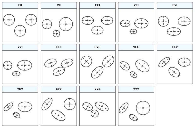
MCLUST models

Notes: E = equal; S=spherical; V=variable; AA=axis-aligned

ID	Volume	Shape	Orientation	Covariance Decomposition	Number of free Covariance parameters
EII	E	S		\(\lambda \mathbf{I}\)	1
VII	V	S		\(\lambda_g \mathbf{I}\)	\(G\)
EEI	E	E	AA	\(\lambda \mathbf{A}\)	\(p\)
VEI	V	E	AA	\(\lambda_g \mathbf{A}\)	\(p+G-1\)
EVI	E	V	AA	\(\lambda \mathbf{A}_g\)	\(pG-G+1\)
VVI	V	V	AA	\(\lambda_g \mathbf{A}_g\)	\(pG\)
EEE	E	E	E	\(\lambda\mathbf{D}\mathbf{A}\mathbf{D}'\)	\(p(p+1)/2\)
EEV	E	E	V	\(\lambda\mathbf{D}_g\mathbf{A}\mathbf{D}'_g\)	\(Gp(p+1)/2-(G-1)p\)
VEV	V	E	V	\(\lambda_g\mathbf{D}_g\mathbf{A}\mathbf{D}'_g\)	\(Gp(p+1)/2-(G-1)(p-1)\)
VVV	V	V	V	\(\lambda_g\mathbf{D}_g\mathbf{A}_g\mathbf{D}'_g\)	\(Gp(p+1)/2\)

MCLUST Cluster Shapes

Cluster shapes that correspond to the covariance structures on the previous slide

Model	Σk	Distribution	Volume	Shape	Orientation
EII	λI	Spherical	Equal	Equal	—
VII	λkI	Spherical	Variable	Equal	—
EEI	λA	Diagonal	Equal	Equal	Coordinate axes
VEI	λkA	Diagonal	Variable	Equal	Coordinate axes
EVI	λAk	Diagonal	Equal	Variable	Coordinate axes
VVI	λkAk	Diagonal	Variable	Variable	Coordinate axes
EEE	λDAD⊤	Ellipsoidal	Equal	Equal	Equal
EVE	λDAkD⊤	Ellipsoidal	Equal	Variable	Equal
VEE	λkDAD⊤	Ellipsoidal	Variable	Equal	Equal
VVE	λkDAkD⊤	Ellipsoidal	Variable	Variable	Equal
EEV	𝜆𝑫𝑘𝑨𝑫⊤𝑘	Ellipsoidal	Equal	Equal	Variable
VEV	𝜆𝑘𝑫𝑘𝑨𝑫⊤𝑘	Ellipsoidal	Variable	Equal	Variable
EVV	𝜆𝑫𝑘𝑨𝑘𝑫⊤𝑘	Ellipsoidal	Equal	Variable	Variable
VVV	𝜆𝑘𝑫𝑘𝑨𝑘𝑫⊤𝑘	Ellipsoidal	Variable	Variable	Variable

MCLUST Cluster Shapes

Cluster shapes that correspond to the covariance structures on the previous slide [source]

faithful finite mixture 2D

mod2 <- Mclust(faithful)
summary(mod2, parameters = TRUE)

---------------------------------------------------- 
Gaussian finite mixture model fitted by EM algorithm 
---------------------------------------------------- 

Mclust EEE (ellipsoidal, equal volume, shape and orientation) model with 3
components: 

 log-likelihood   n df       BIC       ICL
      -1126.326 272 11 -2314.316 -2357.824

Clustering table:
  1   2   3 
 40  97 135 

Mixing probabilities:
        1         2         3 
0.1656784 0.3563696 0.4779520 

Means:
               [,1]      [,2]      [,3]
eruptions  3.793066  2.037596  4.463245
waiting   77.521051 54.491158 80.833439

Variances:
[,,1]
           eruptions    waiting
eruptions 0.07825448  0.4801979
waiting   0.48019785 33.7671464
[,,2]
           eruptions    waiting
eruptions 0.07825448  0.4801979
waiting   0.48019785 33.7671464
[,,3]
           eruptions    waiting
eruptions 0.07825448  0.4801979
waiting   0.48019785 33.7671464

The “best” model is 3 components

This assumes the EEE covariance structure

But how was this determined?

BIC plot

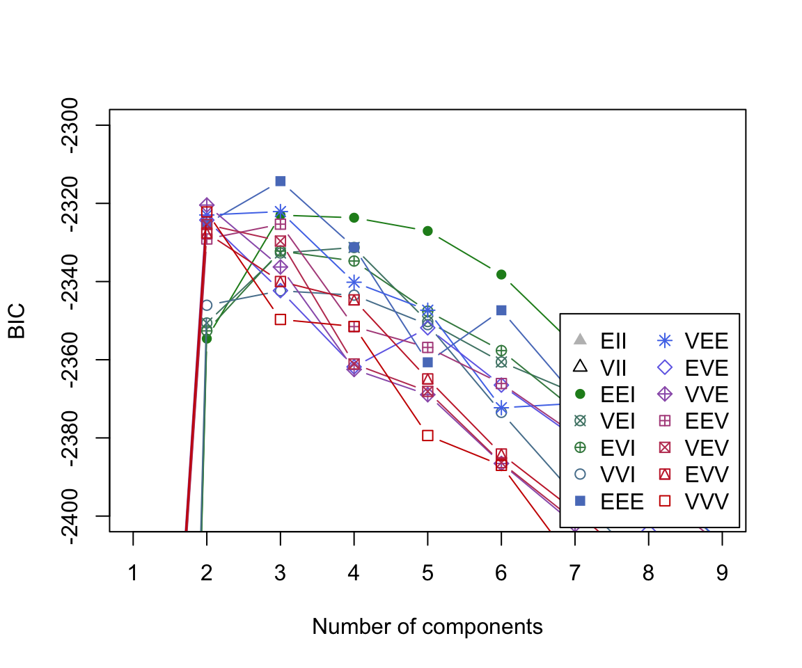
By default, MCLUST will fit a g-component mixture model for all 14 models models for \(g\) = 1, 2, … 9.

For each of these 126 models, a BIC value is calculated.

The BIC

• The Bayesian Information Criterion or BIC (Schwarz, 1978) is one of the most widely known and used tools in statistical model selection. The BIC can be written: \[\begin{equation} \text{BIC} = 2 \ell(x, \hat \theta) - p_f \log{n} \end{equation}\] where \(\ell\) is the log-likelihood, \(\hat \theta\) is the MLE of \(\theta\), \(p_f\) is the # of free parameters and \(n\) is the # of observations.

• It can be shown that the BIC gives consistent estimates of the number of components in a mixtures model under certain regulator conditions (Keribin, 1988 , 2000)

I think this is the non-complete log-like but i’d have to check

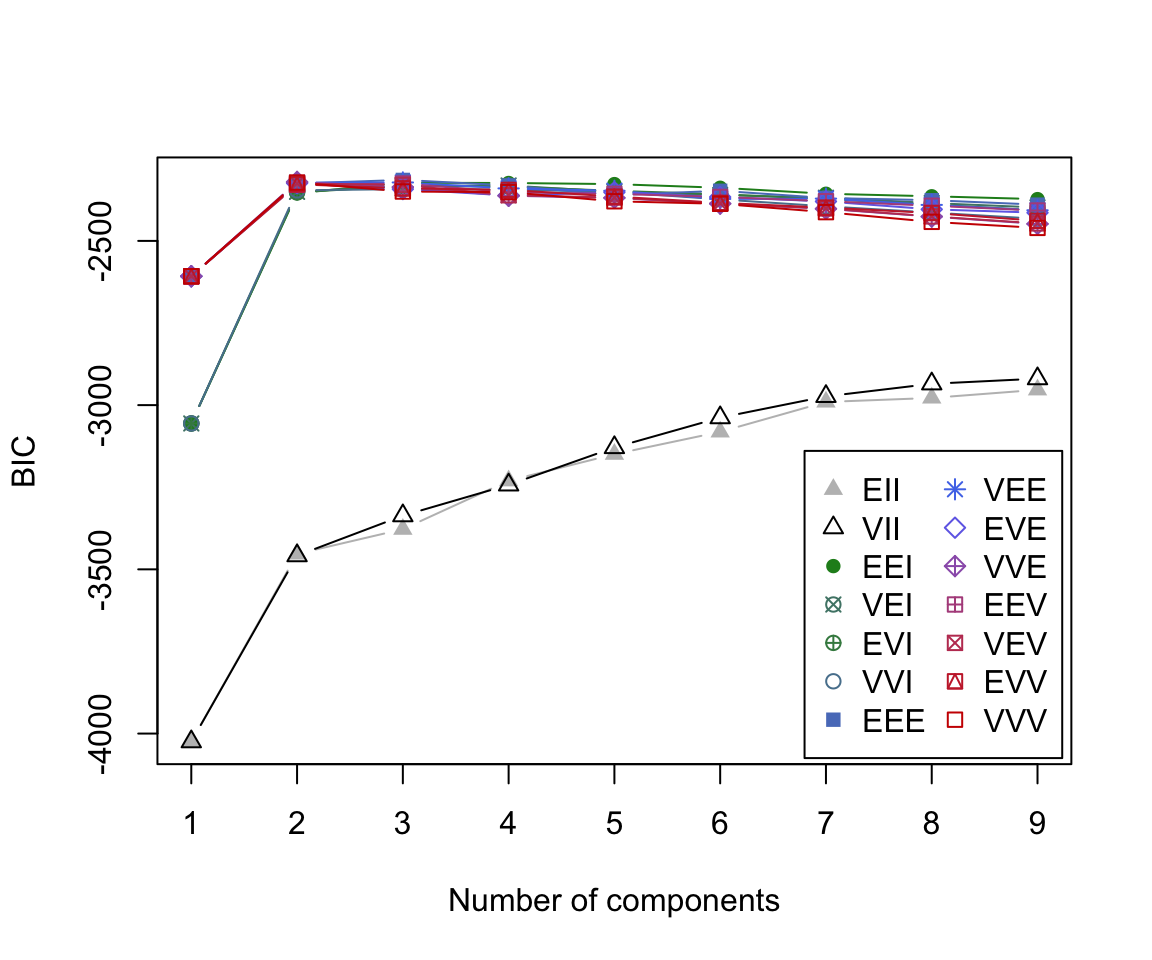
BIC plot (zoomed)

The BIC plot reveals that the model which obtains the largest BIC value is the 3-component mixture model with the ‘EEE’ covariance structure.

as discussed in Problem 2, it is very possible that this is a local (rather than global) maximum

Pros

Why Mixture Model-based Clustering?

• Mathematically and statistically sound using standard theory
• Parameter estimation is built-in, along with number of clusters via model selection
• Provides a probabilistic answer to the question “does observation \(i\) belong to group \(G\)?”
• Adaptable, eg. data with outliers/skewness can be handled by non-Gaussian densities

Cons

Cons (a.k.a. open avenues for research)

• Computationally intensive (takes time to estimate and invert covariance matrices; not feasible for small \(n\) large \(p\) without some decomposition)
• Model-selection method is still viewed as an open problem by many practitioners — BIC grudgingly accepted
• Traditional parameter estimation via EM algorithm prone to local maxima, overconfidence in clustering probabilities, and several other issues

Iris

• Description
• Data frame
• Plot
• Code

Image Source kedro

Here i am using “clusters” as groups of data that clump together, but really these are just know classifcation corresponding to the species are Iris setosa, versicolor, and virginica.

jump to the geyser data set.

We can see that these species form distinct clusters (esp in the Sepal.Width vs Petal.Width scatterplot)

library(ggplot2)
# install.packages("GGally")
library(GGally)

ggpairs(iris,                 # Data frame
        columns = 1:4,        # Columns
        aes(color = Species,  # Color by group (cat. variable)
            alpha = 0.5))     # Transparency 

This famous (Fisher’s or Anderson’s) iris data set gives the measurements in centimeters of the variables sepal length and width and petal length and width, respectively, for 50 flowers from each of 3 species of iris

Mclust

Mclust(data, G = 1:9, modelNames = NULL)

• modelNames when \(n > d\) all avaible models are fit

The best model (as determined by the BIC) is returned:

• modelName A character string denoting the model at which the optimal BIC occurs.

• G The optimal number of mixture components

• parameters:

  • pro for \(\pi_g\)s, $mean for \(\mu_g\)s, $variance for \(\Sigma_g\)s)

library(mclust)

# Load example data
data <- iris[, -5]

# Apply Mclust for clustering
model <- Mclust(data)

# Summary of the model
summary(model)

---------------------------------------------------- 
Gaussian finite mixture model fitted by EM algorithm 
---------------------------------------------------- 

Mclust VEV (ellipsoidal, equal shape) model with 2 components: 

 log-likelihood   n df       BIC       ICL
       -215.726 150 26 -561.7285 -561.7289

Clustering table:
  1   2 
 50 100 

# Visualize results
plot(model, what = "classification")  # Classification plot