Data 311: Machine Learning

👻🎃 Lecture 14: Distance Measures 🎃👻

Dr. Irene Vrbik

University of British Columbia Okanagan

Supervised vs Unsupervised Learning

• Simple methods for modeling a continuous response variable include: regression, KNN-regression, trees, boosting, random forests

• Simple methods for modeling a categorical response variable include: logistic regression, discriminant analysis, KNN-classification, trees, boosting, random forests

• So far we’ve been in the supervised setting where we know the “answers” for response variable \(Y\) which might be continuous (regression) or categorical (classification)

  \[ \begin{align} X &\rightarrow Y \\ \quad \text{input data} &\rightarrow \text{output data (``answers")} \end{align} \]

• Today we move towards unsupervised learning; that is, problems for which we do not have known “answers”.

we don’t have any output values, we’re not try to predict values or labels anymore

so we have a dataset and we usually want to find some structure

In these course we’re going to focus on clustering and dimensionality reduction.

Clustering Problem

We want to find if there are groups (or clusters).

In 2D this might be simple enough,

Recognizing Patterns Looking at the original scatter plot, the human eye naturally tries to make sense of patterns. We instinctively notice clusters or groups of points that seem to be closer together. In this case, there appear to be several distinct regions where points are more densely packed, suggesting natural groupings.

Potential Solution 1

Potential Solution 2

Potential Solution 3

what did we do, we visually inspected which observervations were closer in terms of distance, found the gaps, and

Step 2: Identifying Clusters by Proximity Without any formal rules, we can start grouping points based on their proximity to each other:

There’s a group in the top left where points are close together, creating a loosely defined cluster. Another group appears around the bottom center where points are also densely packed. On the right side, there’s a region with points spread out near each other in a loose grouping.

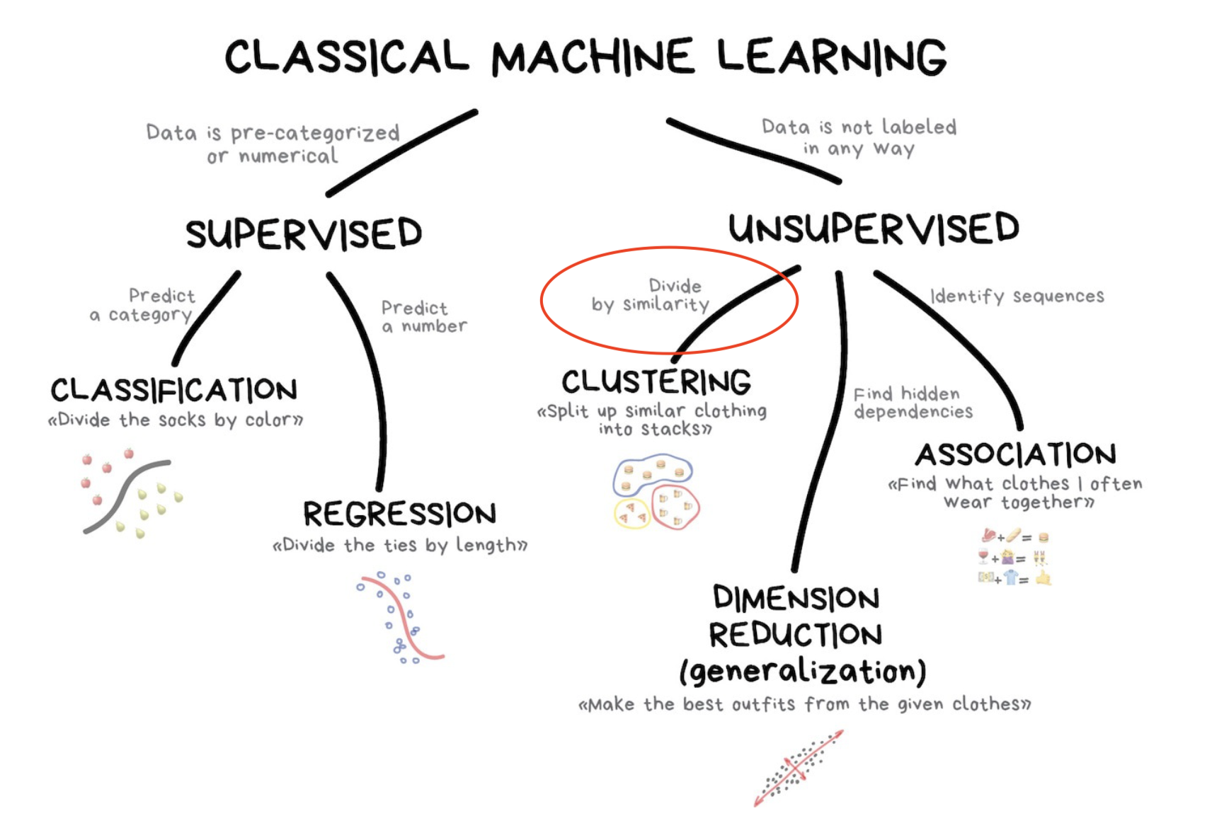
What is Clustering?

• Definition: Clustering is an unsupervised learning technique that groups data points into clusters based on similarity.

• Goal: Identify natural groupings or patterns in data without labeled outcomes.

• Applications: Market segmentation, image analysis, document organization, and anomaly detection.

Unsupervised complications

• How do we define a cluster?
• How do we determine how many clusters are in the data
• Is there any clusters to be found at all?
• How do we compare two different clustering results?

We’ll tackle some of these problems in upcoming lectures but for now let’s talk about …

This is a hard problem to formalize.

many questions arise

with no “answers” we don’t have the usual metrics

Distance

• Prior to diving deep on unsupervised methods, it’s important to note that the vast majority are based on distance calculations (of some form).

• Distance seems like a straightforward idea, but it is actually quite complex …

• For instance, how would the clusetering problem change if we had included some categorical features into the mix?

what if we had in some categorical features - how would that change things?

For more on distance measures see Chapter 3 of Multivariate Statistics with R by Paul J. Hewson

Outline

• Euclidean Distance

• Manhattan Distance

• Mahalanobis Distance

• Matching Binary Distance

• Asymmetric Binary Distance

• Gower’s Distance

Distance Motivation

What is the distance from Trump Tower to Times Square?

• As the crow flies that might be something like 1.1 km

• Restricting ourselves to the sidewalks (walking) its 1.3 km

• Restricting ourselves to car its 1.9km (one way streets)

What is the distance from Trump Tower to UBCO?

In this case we would need to take into account the curvature of the Earth!

• In spaces with curvature, straight lines are replaced by geodesics.

• measurements exist that assume the earth is a sphere

• Talk about McGill research - whats the difference between sequences?

• raman - whats the difference between two raman spectrospy we have these

Euclidean Distance

To begin, we’ll consider that all predictors are numeric. The Euclidean distance between two observations \(x_i\) and \(x_j\) is calculated as \[d^{\text{EUC}}_{ij} = \sqrt{\sum_{k=1}^p (x_{ik} - x_{jk})^2}\]

While simple, it is inappropriate in many settings.

• Euclidean used in knn
• the square root of the squared distance between any two vectors: \(d_{ij} = [(x_i - x_2)^T(x_i - x_2)]^{1/2}\)
  • \(x_i = (x_{i1}, x_{i2}, \dots x_{ip})\)
  • \(x_j = (x_{j1}, x_{j2}, \dots x_{jp})\)
• distance between two p-dimensional points
• readily calculated in R using the dist() with default method = “euclidean”, and daisy() in the cluster pacakge
• see Ch 3 here
• like Pythagus thoerm

where \(x_i = (x_{i1}, x_{i2}, \dots x_{ip})\) and \(x_j = (x_{j1}, x_{j2}, \dots x_{jp})\)

Where Euclidean Fails 1

• Consider the following measurements on people:
  • Height (in cm),
  • Annual salary (in $)
• A $61 difference in annual salary would be considered a minuscule difference, whereas a 61 cm difference in height (approx 2 feet) would be substantial!

• The scale and range of possible values matters
• KNN relies on obs nearest to it, (scale matters).
• large scale variables will have a larger effect on the distance between the observations, than variables that are on a small scale.
• salary will drive the KNN classification results
• futhermore if we give salary in JP Yen

Plotted Euclidean Distance

Is it reasonable to assume A is equidistant (at equal distances) with points B and C?

Scale Matters

• The scale and range of possible values matters!

• If we use a distance-based method, for example KNN, then large scale variables (like salary¹) will have a larger effect on the distance between the observations, than variables that are on a small scale (like height).

• Hence salary will drive the KNN classification results².

1. Imagine if this were in Yen (1 UDS = 149.2 Japanese Yen).

2. see pg 182 in ISLR2 for an example of this

Standardized Euclidean Distance

One solution is to scale the data to have mean 0, variance 1 via \[z_{ik} = \frac{x_{ik}-\mu_k}{\sigma_k}\] Then we can define standardized pairwise distances as \[d^{\text{STA}}_{ij} = \sqrt{\sum_{k=1}^p (z_{ik} - z_{jk})^2}\]

• ie we calculate z-scores
• in practice: \(\mu=\overline x\) and \(\sigma\) is sample sd.
• euclidean distance on z-scores

How it might look after scaling

After scaling those data you might have something more along the lines of this, were C and A are much closer together than A and B

• variance in salary is on the order of tens of thousands
• sd of height is along the lines of 5-10cm
• once we divide by that standard deviation pt c gets moved way closer to a then b will

Manhattan Distance

• Manhattan distance¹ measures pairwise distance as though one could only travel along the axes \[d^{\text{MAN}}_{ij} = \sum_{k=1}^p |x_{ik} - x_{jk}|\]

• Similarly, one might want to consider the standardized form \[d^{\text{MANs}}_{ij} = \sum_{k=1}^p |z_{ik} - z_{jk}|\]

• distance between two points in terms of movements parallel to the axis
• resembles the distance between two points in a city
• Manhattan distance is calculated as the sum of the absolute differences between the two vectors.
• same problem with scale as Euc.
• AKA \(l_1\) norm

1. AKA city-block distance, L1 distance, \(\ell_1\) norm, or Taxicab geometry

Manhattan Visualization

Image sources: Google Maps 2021

• Odd-numbered streets go west and even-numbered streets go east.
• If we can only move in the west and east axis (as is the case for directions on google maps) then we have the manhattan distance

Manhattan Visualization 2

Image Source: and Wikipedia Oct 2022

• The red, yellow, and blue paths all have the same Manhattan distance of 12.

• The green line has Euclidean distance of \(6 \sqrt {2} \approx 8.49\) and is the unique shortest path.

Euclidean Visualization

If we could travel “as the crow flies” then we can make a direct path to Time Square to Trump Tower. (less than the Manhattan distance)

Where Euclidean Fails 2

• Euclidean distance can lead to some misleading results when the variables are highly correlated.

• Let’s consider data simulated from the bivariate normal distribution having

\[\begin{align} \boldsymbol\mu &= \begin{pmatrix} 2 \\ 3 \end{pmatrix} & \boldsymbol\Sigma &= \begin{pmatrix} 5 & 7\\ 7 & 11 \end{pmatrix} \end{align}\]

Simulation

Which point would you consider more unusual? A or B?

• 200 observations

• points fall on a 45 degree angle ellipse

• ellipse is skinny as dictated by our high correlation between x and y

Euclidean Distance for Simulation

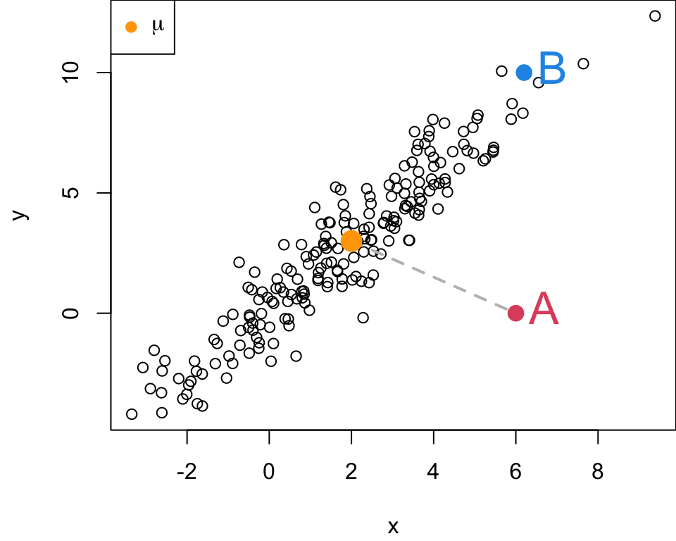
• The euclidean distance between A and \(\mu\) is 5

Euclidean Distance for Simulation

• The euclidean distance between A and \(\mu\) is 5

• The euclidean distance between B and \(\mu\) is 8.16

B is father in terms of Euclidean distance from the center of this distribution, but it is “closer” to the blob of points than A.

Mahalanobis Distance

• Mahalanobis distance takes into account the covariance structure of the data.

• It is easiest defined in matrix form \[d^{\text{MAH}}_{ij} = \sqrt{(x_i - x_j)^\top \boldsymbol{\Sigma}^{-1} (x_i - x_j)}\] where \(^\top\) represents the transpose of a matrix and \(^{-1}\) denotes the inverse of matrix.

• Recall, we saw this distance crop-up in our discussion of LDA/QDA.
• Not only takes into account variance (diagonal) but also covariance (off diagonal) of the data
• can also use for a distribution with \(\mu\) in place of \(x_j\)
• this takes into account the shape of the blob
• works well when two or more variables are highly correlated and even if their scales are not the same

Mahalanobis distance is a generalization of standardized euclidean distance (you can thing of it as standardizing by both variance and covariances).

Mahalanobis Distance for Simulation

• The Mahalanobis distance from point \(\mu\) to A is 64.83

Mahalanobis Distance for Simulation

• The Mahalanobis distance from point \(\mu\) to A is 64.83

• The Mahalanobis distance from point \(\mu\) to B is 4.57

B is closer to \(\mu\) in terms of Mahalanobis distance than A is, despite A being closer to \(\mu\) in terms of Euclidean distance.

Computing Distances in base R:

sum(abs(A - mu)) # Manhattan

[1] 7

Euclidean

sqrt(sum((A - mu)^2))   
sqrt(sum((B - mu)^2)) 
dist(rbind(A,B,mu))
# ^ all pairwise distances

[1] 5
[1] 8.163333
           A         B
B  10.002000          
mu  5.000000  8.163333

Mahalanobis

mahalanobis(A, mu, cov = sigma)
mahalanobis(B, mu, cov = sigma)

[1] 64.83333
[1] 4.573333

## Mahalanobis
t(A - mu)%*%solve(sigma)%*%(A - mu) # returns a 1x1 matrix
t(B - mu)%*%solve(sigma)%*%(B - mu) # returns a 1x1 matrix

See dist(), also the daisy() function in the cluster package

Distances with functions

• The dist() function calculates Euclidean, Manhattan, and other standard distances.

• The daisy() function in R, from the cluster package, calculates dissimilarity matrices for data with mixed types of variables (e.g., numeric, categorical, and ordinal).

data <- matrix(rnorm(10), nrow = 5, ncol = 2); data

           [,1]       [,2]
[1,] -0.2427811  0.9364960
[2,]  0.9093803 -0.4132871
[3,] -1.1053578  1.0853977
[4,] -0.2201988 -0.6779804
[5,] -0.9038184 -0.1437295

Stored as a lower triangular matrix (with all the pairwise distances

we’ll return to daisy() after talking about Gower’s Distance

dist

(dist_matrix <- dist(data, method = "euclidean"))

          1         2         3         4
2 1.7746522                              
3 0.8753343 2.5110209                    
4 1.6146343 1.1601774 1.9730709          
5 1.2664350 1.8331260 1.2455408 0.8676173

(dist_matrix <- dist(data, method = "manhattan"))

         1        2        3        4
2 2.501945                           
3 1.011478 3.513423                  
4 1.637059 1.394272 2.648537         
5 1.741263 2.082756 1.430667 1.217870

displaying it as a lower triangle avoids redundancies since the dist between A and B is the same as B and A

The structure of the output is an object of class dist: a lower triangular matrix showing pairwise distances.

Standardization

To standardize our data, we can use the scale() function.

(strzd_data = scale(data))

            [,1]       [,2]
[1,]  0.08853014  0.9696640
[2,]  1.55040596 -0.7102335
[3,] -1.00591718  1.1549824
[4,]  0.11718278 -1.0396623
[5,] -0.75020170 -0.3747505
attr(,"scaled:center")
[1] -0.3125551  0.1573794
attr(,"scaled:scale")
[1] 0.7881390 0.8034914

So our standardized Euclidean distance can be found using

dist(strzd_data, 
     method = "euclidean")

         1        2        3        4
2 2.226912                           
3 1.110026 3.164462                  
4 2.009531 1.470596 2.465323         
5 1.584589 2.324940 1.550959 1.092915

When to Standardize?

• This brings us to an important question…when should we use a standardized measure, and when should we not?

• It is often a good idea, and generally necessary if measurements are on vastly different units.

• Unless you have a good reason to believe that higher variance measures should be weighted heavier, then you probably want to standardize in some form.

• some methods will standardize “underneath the hood” for us by default
• some unsupervised methods are scale invariant, in which case you don’t have to worry about it.
• measurements on different units? Rule of thumb is to standardize

In fact, a lot of machine learning algorithms will scale by default. e.g., kmeans(), pca(), svm() (e1071 package), neuralnet() (keras package)

iClicker

iClicker: Mahalanobis

Which of the following is a key feature of Mahalanobis distance?

1. It considers only the variances of each feature.
2. It can handle both numeric and categorical features.
3. It only works with binary features.
4. It accounts for both variances and covariances between features.

From Numeric to Mixed

• What if some/all the predictors are not numeric?

• We can consider several methods for calculating distances based on matching.

• For binary data case, we can get a “match” either with a 1-1 agreement or 0-0.

Matching Binary Distance

• We can actually define another matching method that is equivalent to Manhattan/city-block,

\[d^{\text{MAT}}_{ij} = \text{\# of variables with opposite value}\]

• This is simple sum of disagreements is the unstandardized version of the M-coefficient.

• Let’s see an example,…

• this is the unscaled version of the M-coef

President Example

Let’s look at some binary variables for US presidents:

• Democrat logical indicating if they are a democrat
• Govenor logical indicating if they were they formerly a governor 1 = yes
• VP logical indicating if they were formerly a vice president
• 2nd Term logical indicating if they serve a second term
• From Iowa logical indicating if they are originally from Iowa

Distance between Bush and Obama

	Democrat	Governor	VP	2nd Term	From Iowa
GWBush	0	1	0	1	0
Obama	1	0	0	1	0
Trump	0	0	0	0	0

The Manhattan distance between GWBush vs Obama: \[|0-1|+|1-0|+|0-0|+|1-1|+|0-0| = 2\]

This is equivalent to the Matching Binary Distance since they do not match in two variables: Democrat and Governor. \[ d^{\text{MAT}}_{12} = \text{\# of variables with opposite value} = 2 \]

M-coefficient

• The M-coefficient (or matching coefficient) is simply the proportion of variables in disagreement in two objects over the total number of variable comparisons, p.

• To put another way, you can think of Matching Binary Distance as an unscaled version of the M-coefficient.

\[ \begin{equation} d_{12}^{\text{M-coef}} = \frac{d_{12}^{MAT}}{p} = \frac{2}{5} = 0.4 \end{equation} \]

• Binary distance measures are often divided by the number of predictors p for simplier interpretations
• in binary its often call matching
• counting the number of variables with the same value
• (or 1 - proportion of variables with opposite values)
• M-ceof == simple matching ceofficient

Calculate M-coefficient

	Democrat	Governor	VP	2nd Term	From Iowa
GWBush	0	1	0	1	0
Obama	1	0	0	1	0
Trump	0	0	0	0	0

Calculating the simple matching M-coefficient¹ \[d^{\text{M-coef}}_{12} = \frac{\text{\# of disagreements}}{p} = \frac{2}{5} = 0.4\]

• so here we have 3 matches and 2 disagreements
• often for binary distance measures is we divide by the number of predictors for simple interpretation
• on 40% of the variables considered, the presidents do not match

1. The closely related Jaccard’s coefficient only counts 1-1s as matches

Question: Do you think a 0-0 match in From Iowa should really map to a binary distance of 0?

	Democrat	Governor	VP	2nd Term	From Iowa
GWBush	0	1	0	1	0
Obama	1	0	0	1	0
Trump	0	0	0	0	0

Since a 0-0 “match” does not imply that they are from similar places in the US, I would argue not.

• 2nd term 1-1 match is straight forward. They both served a second term so they don’t differ on that predictor. (distance contribution of 0)
• 0-0 mathc on Iowa is less straightforward
• VP 0-0 is less clear but if it’s trying to determine if the individual was in politics before their presidency a 0-0 match would be misleading (Obama was a prof but was also a senator)
• President George W bush was from New Haven, Connecticut
• President Barack Obama was form Honolulu, Hawaii

Asymmetric Binary Distance

• For reasons discussed on the previous slide, it makes sense to toss out those 0-0 matches.

• In this case, what we would be considering is asymmetric binary distance

\[d^{\text{ASY}}_{ij} = \frac{\text{\# of 0-1 or 1-0 pairs}}{\text{\# of 0-1, 1-0, or 1-1 pairs}}\]

numerator: the number of things that don’t match

denom: the total number of pairs that aren’t 0-0

• asymetric can also mean dis(0,1) \(\neq\) dist(1,0)

Calculate Asymmetric Distance

	Democrat	Governor	VP	2nd Term	From Iowa
GWBush	0	1	0	1	0
Obama	1	0	0	1	0
Trump	0	0	0	0	0

The asymmetric binary distance between Bush and Obama:

\[ \begin{align} d^{\text{ASY}}_{ij} &= \frac{\text{\# of 0-1 or 1-0 pairs}}{\text{\# of 0-1, 1-0, or 1-1 pairs}}= \frac{2}{3} = 0.67 \end{align} \]

• most software will allow you to specify on a case-to-case basis whether you would like it to be treated as asymmetric or not
• don’t necessarily have to say all zero zero matches are tossed out
  • eg. count VP 0-0 as match but not from iowna
• so 2/4 if we wanted to count VP 0-0 as matches

iClicker

Asymmetric Binary Distance

Which of the following best describes the Asymmetric Binary Distance

1. It ignores 0-0 matches when calculating the distance between two binary vectors.
2. It calculates the number of matching variables divided by the total number of variables.
3. It only considers Euclidean distances on standardized binary data.
4. It includes 0-0 matches to fully count the differences between two binary vectors.

Distance for Qualitative Variables

• For categorical variables having \(>2\) levels, a common measure is essentially standardized matching once again.

• If \(u\) is the number of variables that match between observations \(i\) and \(j\) and \(p\) is the total number of variables, the measure¹ is calculated as: \[d^{\text{CAT}}_{ij} = 1 - \frac{u}{p}\]

• basically a standardized form of matching
• can be performed by daisy()
• bc we are counting the matches we’re going to subtract this ratio from 1
• most commonly specified this saw

1. It is invariant to the codings used or the order of the levels of the factor and can be calculated using the R function daisy() function in the class package.

Distance for Mixed Variables

• But often data has a mix of variable types.

• Gower’s distance is a common choice for computing pairwise distances in this case.

• The basic idea is to standardize each variable’s contribution to the distance between 0 and 1, and then sum them up.

• talk about one method

• that we can use that can combine all of numeric categorical and continuous

• One possible use of Gower distance is with k-means clustering with mixed data because k-means needs the numeric distance between data items.

Aside ordinal variables most common way to be would be to treat it as a continuous

Gower’s Distance

Gower’s distance (or Gower’s dissimilarity) is calculated as: \[d^{\text{GOW}}_{ij} = \frac{\sum_{k=1}^p \delta_{ijk} d_{ijk}}{\sum_{k=1}^p \delta_{ijk}}\]

where

• \(\delta_{ijk}\) = 1 if both \(x_{ik}\) and \(x_{jk}\) are non-missing¹ (0 otherwise),
  
• \(d_{ijk}\) depends on variable type

• sum the individual similarities (however calculated) and divide them by the total number of applicable comparisons
• If the element is numeric, the term is the absolute value of the difference divided by the range.
• If the element is non-numeric the term is 1 if the elements are different or the term is 0 if the elements are the same. The Gower distance is the average of the terms.
• average of the (known) “scores”

1. a 0-0 binary match is often counted as “missing” to match asymmetric binary

• Quantitative numeric \[d_{ijk} = \frac{|x_{ik} - x_{jk}|}{\text{range of variable k}}\]

• Qualitative (nominal, categorical) \[d_{ijk} = \begin{cases} 0 &\text{ if obs $i$ and $j$ agree on variable $k$, } \\ 1 &\text{ otherwise} \end{cases} \]

• Binary \(d_{ijk} = \begin{cases} 0 & \text{ if obs $i$ and $j$ are a 1-1 match, } \\ 1 &\text{ otherwise} \end{cases}\)

Quatitiative

• This is essentially the City Block distance with the extra assumption that all variables had first been standardised by dividing by their range first - for qualitative and binary we are just back to matching

• range-normalized manhattan distance

Notice that each individual term will be between 0.0 and 1.0 inclusive, therefore the Gower distance will always be between 0.0 and 1.0 where a distance of 0.0 means the two items are the same and a distance of 1.0 means the two items are as far apart as possible, relative to the source dataset.

Example of Gower’s Distance

	Party	Height (cm)	Eye Colour	2 Terms	From Iowa
Biden	Democratic	182	Blue	No	No
Trump	Republican	188	Blue	NA	No
Obama	Democratic	185	Brown	Yes	No
Fillmore	Third Party	175	Blue	No	No

• 13th presdient Fillmore has a 3rd-party affiliation
• variable not be binary
• this is important because we need to know the range of the continuous predictors to calculate Gowers distance

We assume we have this data for all past and present US presidents; if you don’t like this example, you can see another example here

Distance between Biden and Trump

0-0 pairs not counted as matches

We will not consider 0-0 to be matches.

\(k\)	\(\delta_{12k}\)	\(d_{12k}\)	\(\delta_{12k}d_{12k}\)
Party	1
Height	1
EyeColour	1
2 Terms	0
Iowa	0

Party Calculations

	Party	Height (cm)	Eye Colour	2 Terms	From Iowa
Biden	Democratic	182	Blue	No	No
Trump	Republican	188	Blue	NA	No

\(k\)	\(\delta_{12k}\)	\(d_{12k}\)	\(\delta_{12k}d_{12k}\)
Party	1	1	1
Height	1
EyeColour	1
2 Terms	0
Iowa	0

Since Biden (\(i = 1\)) and Trump’s (\(j = 2\)) political parties don’t match (Democratic \(\neq\) Republican) this \(d_{12}\) is 1.

Range of Presidents Heights

To calculate \(d_{12k}\) we need the range of the Height(cm)s

• Tallest President: Abraham Lincoln at 193 centimeters
• Shortest President: James Madison at 163 centimeters

Range of Height variable (\(k = 2\)) is 193-163 = 30

\(d_{1,2,2} = \dfrac{|x_{ik} - x_{jk}|}{\text{range of variable k}} = \dfrac{|188 - 182|}{30} = 0.2\)

• James Madison 4th US president from 1809 to 1817

Height Calculations

	Party	Height (cm)	Eye Colour	2 Terms	From Iowa
Biden	Democratic	182	Blue	No	No
Trump	Republican	188	Blue	NA	No

\(k\)	\(\delta_{12k}\)	\(d_{12k}\)	\(\delta_{12k}d_{12k}\)
Party	1	1	1
Height	1	0.2	0.2
EyeColour	1
2 Terms	0
Iowa	0

EyeColour Calculations

	Party	Height (cm)	Eye Colour	2 Terms	From Iowa
Biden	Democratic	182	Blue	No	No
Trump	Republican	188	Blue	NA	No

\(k\)	\(\delta_{12k}\)	\(d_{12k}\)	\(\delta_{12k}d_{12k}\)
Party	1	1	1
Height	1	0.2	0.2
EyeColour	1	0	0
2 Terms	0
Iowa	0

2 Terms Calculations

	Party	Height (cm)	Eye Colour	2 Terms	From Iowa
Biden	Democratic	182	Blue	No	No
Trump	Republican	188	Blue	NA	No

\(k\)	\(\delta_{12k}\)	\(d_{12k}\)	\(\delta_{12k}d_{12k}\)
Party	1	1	1
Height	1	0.2	0.2
EyeColour	1	0	0
2 Terms	0	-	0
Iowa	0

From Iowa Calculations

	Party	Height (cm)	Eye Colour	2 Terms	From Iowa
Biden	Democratic	182	Blue	No	No
Trump	Republican	188	Blue	NA	No

\(k\)	\(\delta_{12k}\)	\(d_{12k}\)	\(\delta_{12k}d_{12k}\)
Party	1	1	1
Height	1	0.2	0.2
EyeColour	1	0	0
2 Terms	0	-	0
Iowa	0	0	0

Gower’s Distance Calculation

\(k\)	\(\delta_{12k}\)	\(d_{12k}\)	\(\delta_{12k}d_{12k}\)
Party	1	1	1
Height	1	0.2	0.2
EyeColour	1	0	0
2 Terms	0	-	0
Iowa	0	0	0
Total	3		1.2

\[ d^{\text{GOW}}_{ij} = \frac{\sum_{k=1}^p \delta_{ijk} d_{ijk}}{\sum_{k=1}^p \delta_{ijk}} = \frac{1.2}{3} = 0.4 \]

daisy

library(cluster)
data <- data.frame(
  x1 = factor(c("A", "B", "A", "B")),
  x2 = c(1.2, 3.4, 2.3, 4.5),
  x3 = ordered(c("Low", "Medium", "High", "Medium")))

print(data)

  x1  x2     x3
1  A 1.2    Low
2  B 3.4 Medium
3  A 2.3   High
4  B 4.5 Medium

 daisy(data, metric = "gower")

Dissimilarities :
          1         2         3
2 0.7222222                    
3 0.2777778 0.7777778          
4 0.8333333 0.1111111 0.8888889

Metric :  mixed ;  Types = N, I, O 
Number of objects : 4

Comments

• Gower distance will always be between 0.0 and 1.0

  • a distance of 0.0 means the two observations are identical for all non-missing predictors

  • a distance of 1.0 means the two observations are as far apart as possible for that data set

• The Gower distance can be used with purely numeric or purely non-numeric data, but for such scenarios there are better distance metrics available.

• There are several variations of the Gower distance, so if you encounter it, you should read the documentation carefully.

• Notice that each individual term will be between 0.0 and 1.0 inclusive, therefore the Gower d will alwasy be between 0 and 1
• sidenote: oridinal data are usually just treated as a number