Data 311: Machine Learning

Lecture 13: Regularization in Regression (Ridge Regression and LASSO)

Dr. Irene Vrbik

University of British Columbia Okanagan

Learning Objectives

• Goal: Understand the concept of regularization and its role in regression.

• Objectives:

  • Explain overfitting in regression models.

  • Describe L1 regularization (aka Lasso) and L2 Regularization (aka Ridge Regression)

  • Implement LASSO and Ridge Regression to improve model generalization.

Recall: Linear Model

Recall the linear model:

\[ Y = \beta_0 + \beta_1 X_1 + ··· + \beta_p X_p + \epsilon \]

In ordinary least squares regression, estimates of the regression coefficients (i.e. the \(\beta\)s) are found by minimizing the residuals sum of squares (RSS) (this as our “cost” function)

\[RSS = \sum_{i=1}^n (y_i - \hat y_i)^2\]

• OLS may not be the best model
• we discuss some ways in which the simple linear model can be improved improved by replacing ordinary least squares fitting with some alternative fitting procedures.

Recap

• We’ve now seen a couple of alternatives to the linear model for regression.

• BUT, the linear model still reigns supreme in most realms of science due to its simplicity (which helps for inference).

• We can improve upon the linear model (both in terms of prediction accuracy and model interpretibility) by replacing ordinary least squares fitting with some alternative fitting procedures: shrinkage (aka regularization) methods.

• The are simple, easy to interpret and work well
• one of these models will perform feature selection for us (which is important when we risk overfitting and makes it easier to interpret and more useful)

Motivation

• Overfitting

• Multicollinearity

• Feature Selection

• Enhanced Interpretability

• Improving Prediction Accuracy

Overfitting

• In regression the following can lead to overfitting:

  • high-dimensional¹ data (e.g. \(p>n\)),
  • too many predictors and/or interactions
  • too complexity (e.g. high-degree polynomial)

• Shrinkage methods (Ridge and LASSO) discourages overly complex models and reduces variance, leading to better generalization on test data.

It’s becoming more and more common that \(p > n\)

overfitting: where the model captures noise rather than the underlying pattern. This often results in high variance and poor predictive performance on new data.

1. when the number of predictors \(p\) is greater than the number of observations \(n\) it impossible to obtain unique estimates for the regression coefficients with OLS.

Non-unique solutions

Think about fitting a OLS line to a single observation.

Non-unique solutions

Think about fitting a OLS line to a single observation.

• This line has a 0 SSR

Non-unique solutions

Think about fitting a OLS line to a single observation.

• This line has a 0 SSR
• As does this one

Non-unique solutions

Think about fitting a OLS line to a single observation.

• This line has a 0 SSR
• As does this one
• As does this one

High Variance (small \(n\))

Think about fitting a OLS line to two data points

• This line has a 0 SSR
• It has high variance
• And low bias

High variance typically happens when the amount of data is very limited relative to the number of predictors or model complexity.

• When the dataset is very small, a regression model (even a simple one) can become highly responsive to the few data points it has.

• this line has high variance (two other random points from my training set would lead to very different line)

• we know that this model where the number of parameters \(\beta_0\), and \(\beta_1\) = number of observations is overfitting

More examples:

• High Dimensionality: \(p\approxeq n\) or \(p>n\)

• more complex models: More complex regression models

Overfitting (Complexity)

Higher degree polynomials are clearly overfitting to the data - it captures the noise in the training data, leading to poor predictions on new data.

We see that, as M (the degree) increases, the magnitude of the coefficients typically gets larger. This happens often.

• In particular for the M = 9 polynomial, the coefficients have become finely tuned to the data by developing large positive and negative values and these compensate with one another so you get exact fits to the data.

Point: one way that this overfitting manifests itself is that the magnitued of these estimated coefficients get quite big

	Degree = 1	Degree = 3	Degree = 9
\(\hat \beta_0\)	0.53	-0.197	0
\(\hat \beta_1\)	0.171	2.057	71
\(\hat \beta_2\)		-0.862	-474
\(\hat \beta_3\)		0.084	1317
\(\hat \beta_4\)			-1974
\(\hat \beta_5\)			1754
\(\hat \beta_6\)			-950
\(\hat \beta_7\)			307
\(\hat \beta_8\)			-54
\(\hat \beta_9\)			4

Notice how the coefficients get really large

The estimated polynomial regression coefficients for Degrees 1, 3, and 9.

Bias-Variance Tradeoff

An overfitted regression model has high complexity relative to the amount of data available, which leads to poor generalization on new data.

• more generally, when \(p > n\) estimates may have high variance
• this leads to unreliable predictions
• why? see plot

Combating High Variance

Instead of least squares, we will consider an alternative fitting procedure that will introduce a small amount of bias to get back a significant drop in variance (thereby improving prediction accuracy).

read caption

Multicollinearity

• When predictors are highly correlated, OLS regression may yield large and unstable coefficients, as it cannot distinguish the individual effects of each predictor.

• Ridge regression is particularly useful for addressing multicollinearity by penalizing large coefficients, making the estimates more stable and reliable.

• LASSO can even set some coefficients to zero, effectively selecting a subset of predictors, which is useful in highly collinear datasets.

Feature Selection

• We’ve look at some crude feature selection methods previously (e.g. forward and backward selection; variable importance from trees).

• LASSO provides an automatic feature selection by shrinking some coefficients to zero.

• This allows for a more parsimonious¹ model.

• To combat this, we could use subset selection² wherein only a subset of the \(p\) predictors that we believe to be related to the response are used to fit the model (see Ch 6.1 in ISLR)

• Using cross-validated prediction error, for example, we could select a single best model from all possible models.

• For large \(p\), however, an exhaustive search of every possible subset of predictors is not computationally feasible³; furthermore it will be liable to overfit to the data.

• subset selection requires fitting \(2^p\) models (\(p\) = 10 means 1024 models, \(p = 40\) 1,099,512,000,000 over 1 trillion models).

• So we can pick the best model with \(k\) predictors by choosing the one that has the smallest test error

• authors suggest to only use this if you have a handful or two of predictors

• ridge regression and the lasso can be interpreted as computationally feasible alternatives to best subset selection

1. a parsimonious model is one that achieves its objective with the simplest possible structure

2. e.g. forward, backward, and mixed-stepwise selection

3. there are \({p \choose k}\) possible ways of choosing \(k\) predictors from \(p\) predictors

Enhanced Interpretability

• With many predictors, some of which may be irrelevant, OLS can become inefficient and harder to interpret.

• By focusing only on the most relevant predictors, our model becomes easier to interpret

• This is particularly valuable in fields where interpretability is crucial, such as medical research or finance.

Improving Prediction Accuracy

• Shrinkage methods can improve the predictive accuracy of a regression model by balancing the tradeoff between bias and variance.

• By introducing a small amount of bias (penalizing coefficients), we can significantly reduce variance, leading to a lower MSE on new data compared to OLS.

  🤓 One can prove that if \(\mathbf{X}^T\mathbf{X}\) is full rank¹, then using some amount of regularization still improves the model (Hoerl and Kennard’s, 1970)

Full rank is am important condition for obtaining a unique solution in ordinary least squares (OLS) regression.

OLS will always be worse (at least a little bit) than regularization.

• when \(p >n\) estimates of coefficients become unstable and can vary significantly with minor changes in the data.
• high variance –> unreliable predictions
• one solution to the \(p>n\) problem is to reduce the number of features.
• while this can improve in terms of prediction accuracy it also has the benefit of improving …

1. when \(n > p\) and there are no redundant (or perfectly collinear) predictors in \(\mathbf{X}\)

Model: Matrix Representation

\[\begin{align} f(x_i) &= \beta_0 + \beta_1 x_{i1}+ \beta_2 x_{i2} + \dots + \beta_p x_{ip}\\ &= \beta^\top x_i = \begin{pmatrix} \beta_0 & \dots & \beta_p \end{pmatrix} \begin{pmatrix} x_{i0} \\ x_{i1} \\ \vdots \\ x_{ip} \end{pmatrix} \end{align}\]

where \(x_{i0} := 1\) and \(x_i\) is the vector of all observed

predictors for observation \(i\) \[ \mathbf{X} = \begin{pmatrix} x_0^\top \\ x_1^\top \\ \vdots \\ x_n^\top\\ \end{pmatrix} = \begin{pmatrix} 1 & x_{11}& x_{12} & \dots & x_{1p} \\ 1 & x_{21}& x_{22} & \dots & x_{2p} \\ \vdots & \vdots & \ddots & \vdots \\ 1 &x_{n1} & x_{n2} & \dots & x_{np} \end{pmatrix} = \begin{pmatrix} \mathbf{x}_0 & \mathbf{x}_1 & \dots & \mathbf{x}_p \end{pmatrix} \]

Loss: Matrix Representation

Using this notation, the loss function becomes

\[\begin{align*} \mathcal{L}(\beta) &= \frac{1}{n} \sum_{i=1}^{n} \left( y_i - \beta^\top x_i \right)^2 \\ &=\frac{1}{n}(\mathbf{y} - \mathbf{X} \beta )^\top ( \mathbf{y} - \mathbf{X} \beta )\\ &= \frac{1}{n} \| \mathbf{y} - \mathbf{X} \beta \|^2. \end{align*}\]

where \(\| v \|\) is the Euclidean norm (or \(\ell_2\) norm) of vector \(v\).

\[\begin{align} \begin{pmatrix} \beta_0 & \dots & \beta_p \end{pmatrix} \begin{pmatrix} 1 \\ x_{i1} \\ \vdots \\ x_{ip} \end{pmatrix} \end{align}\]

Lp-norms

The p-norm (or \(\ell_p\)/Lp norm) is defined as: \[ || x ||_p = \left(\sum_i |x_i|^p\right)^{1/p} \]

where \(x\) is a of vector \(\mathbf {x} =(x_{1},\ldots ,x_{n})\)

Hence the squared l2-norm is just the sum of squares

The \(\ell_2\)-norm is Euclidean distance, \(|| x ||_2 = \sqrt{\left(\sum_i x_i^2\right)} = \sqrt{x_1^2 + x_2^2 + \ldots + x_i^2}\)

The \(\ell_1\)-norm is the Manhattan distance \(|| x ||_1 = \sum_i |x_i| = |x_1| + |x_2| + \ldots + |x_i|\)

Regularization

Regularizes regression uses the following cost function:

\[\begin{align*} \mathcal{L}(\beta) &= \frac{1}{n} \| \mathbf{y} - \mathbf{X} \beta \|^2 \textcolor{purple}{ + \lambda R(\beta)} \end{align*}\] where \(\textcolor{purple}{\lambda R(\beta)}\) is a penalty term and \(\lambda\) is a regularization parameter (aka a tuning parameter)

Two types

There are two common approaches to regularization

Ridge regression (L2-norm)

\[ \begin{align} R(\beta) &= \| \beta \|^2 \\ &= \sum_j \beta_j^2 \end{align} \]

LASSO (L1-norm)

\[ \begin{align} R(\beta) &= \| \beta \|_1 \\ &= \sum_j | \beta_j | \end{align} \]

Elastic net uses:

\[ \lambda_1 \| \beta \|_1 + \lambda_2 \| \beta \|^2_2 \]

When a norm is written without a subscript, it generally refers to the L2 norm (also known as the Euclidean norm) by default

Ridge Regression

Ridge regression (RR) includes a penalty in the estimation process and aims to minimize:

\[\begin{align*} \mathcal{L}(\beta) &= \frac{1}{n} \| \mathbf{y} - \mathbf{X} \beta \|^2 \textcolor{purple}{ + \lambda \| \beta \|^2} \end{align*}\] An equivalent way to write this is: \[ RSS + \lambda \sum_{j=1}^p \beta_j^2 \]

where \(\lambda \geq 0\) is a tuning parameter that shrinks the \(\beta_j\) estimates towards 0.

• this is going to penalize coefficients that are too large
• we pay a price for non-zero coefficents
• that price gets bigger as \(\beta_j\) gets bigger
• notice how \(\beta_0\) is omitted since it wouldn’t make sense to penalize that magnitude

Similar to the penalty in cross-complexity pruning!

• this is going to penalize coefficients that are too large
• we pay a price for non-zero coefficents
• that price gets bigger as \(\beta_j\) gets bigger
• notice how \(\beta_0\) is omitted since it wouldn’t make sense to penalize that magnitude

L2 Regularization

The squared L2 norm in used in the Ridge Regression penalty:

\[ \lambda || \beta ||_2^2 = \lambda \sqrt{ \beta_1^2 + \beta_2^2 + \ldots + \beta_p^2 }^2 = \lambda\sum_{i=1}^p \beta_i^2 \]

• This process of adding a norm to our cost function is known as regularization.

• Hence this Ridge Regression is also known as L2 regularization.

• where \(\hat \beta\) denotes the vector of least squares coefficient estimates
• $|| ||_2 $ measures the distance of \(\hat \beta\) from zero

Lasso

The least absolute shrinkage and selection operator or LASSO is arguably the most popular modern method applied to linear models. It is quite similar to Ridge only now it minimizes \[\begin{align*} RSS + \lambda \sum_{j=1}^p |\beta_j| \end{align*}\]

Important advantage

LASSO will force some coefficients to 0 (whereas RR will only force them “close” to 0)

• where \(\lambda\) is a tuning parameter.
• \(\beta_j^2\) is replaced with \(|\beta_j|\)
• so it is performing variable selection
• Tibshirani invented it.
  

L1 regularization

Another way that you might see this model being presented is using the L1 norm; in other words, the LASSO uses the \(\ell_1\) penalty:

\[ \begin{align} \lambda || \beta ||_1 &= \lambda\left( | \beta_1 | + | \beta_2 | + \ldots + | \beta_p | \right)\\ &= \lambda\sum_{i=1}^p | \beta_i | \end{align} \]

Hence this method is also referred to as L1 regularization.

Shrinkage penalty

so the model will pay the price for large in magnitue coefficients

Going back to our motivating examples, we know this can be very helpful for models where we are overfitting

\(\lambda \sum_{j=1}^p \beta_j^2\) is the shrinkage penalty that will penalize the model for the total “size” of the coefficients¹

• As \(\lambda\) increases the coefficient estimates will tend to “shrink” towards 0.
• The penalty will be small when \(\beta_1, \dots \beta_p\) are close to zero
• Hence minimizing \(RSS + \lambda \sum_{j=1}^p \beta_j^2\) will encourage smaller (in magnitude) values for \(\beta_j\)

• λ controls the relative impact of this penalty on RSS
• Not unlike the cross complexity tuning we did for trees (where the penalty was \(\alpha\) times the size of the tree (terminal nodes))
• now instead of the number of the terminal nodes paying a cost, is the magnitude of the coefficients

The model will prefer model with small coefficients, which in turn means that it will prefer simplier models

This is a way of formalizing the parsimony concept that prefers simpler models to more complicated models taht fit the data similarly well.

1. the shrinkage penalty is not applied to the intercept \(\beta_0\)

Tuning Parameter

• Clearly our choice for \(\lambda\) will be an important one (can you guess how we will find it?)

• If \(\lambda=0\) then the estimation process is simply least squares.

• As \(\lambda\) increases, the flexibility of the ridge regression fit decreases, leading to decreased variance but increased bias.

• As \(\lambda \rightarrow \infty\) then the penalty grows and the coefficients approach (but never equal) 0; this corresponds to the null model that contains no predictors.

Like a knob

• Clearly, some care is required in determining \(\lambda\).
• lambda encourages parametesr to be “shrunk” towards 0.
• how pushy it is will depend on the size of lambda
• recall if \(\beta_j\) is 0 then \(X_j\) doesn’t appear in the model
• tradeoff between fit and size of the coefs
• note familiarity with trees

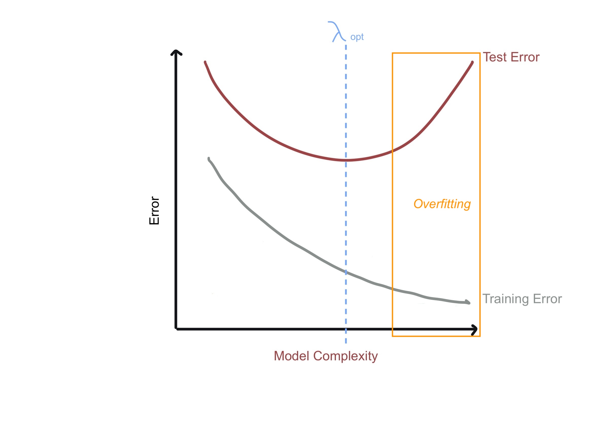
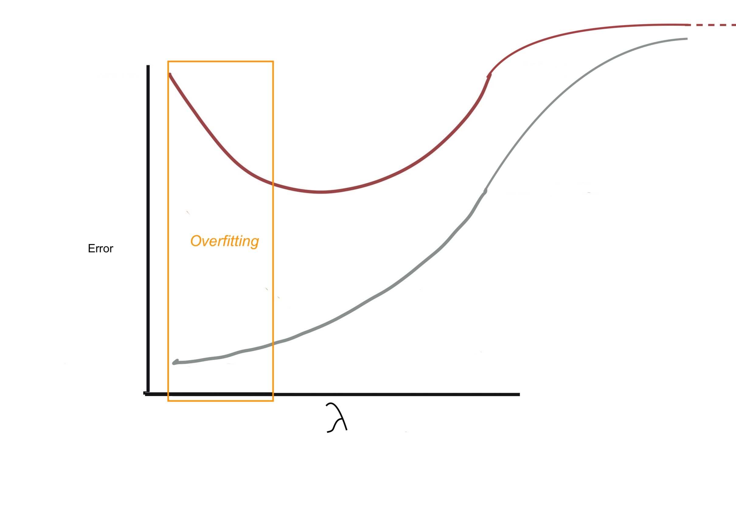
Imagine we have some regression model that is overfitting. Through regularization we aim add some bias to some bias to the model thereby decreasing variance and moving us from the overfitting zone to an optimal zone

High-level conceptual model.

How do you think we’re going to find this optimal?

Note that when you are reading the following plots the horizontal-axis will represent the value of \(\lambda\). The overfitting zone corresponds to small values of \(\lambda\). N.B. when \(\lambda =0\) no regularization is being performed (i.e. OLS regression). When \(\lambda \rightarrow \infty\) we have the null model

Example: Credit

The Credit dataset contains information about credit card card holders and includes 11 variables including:

• Balance the average credit card debt for each individual (response) and several quantitative predictors:

  • Age, Cards (number of credit cards), Education (years of education), Income (in thousands of dollars), Limit (credit limit), and Rating (credit rating).

Fitting a least squares regression model to this data, we get…

MLR Credit fit

library(ISLR2); data(Credit)
lfit <- lm(Balance~., data = Credit)
(sfit <- summary(lfit))

...
              Estimate Std. Error t value Pr(>|t|)    
(Intercept) -479.20787   35.77394 -13.395  < 2e-16 ***
Income        -7.80310    0.23423 -33.314  < 2e-16 ***
Limit          0.19091    0.03278   5.824 1.21e-08 ***
Rating         1.13653    0.49089   2.315   0.0211 *  
Cards         17.72448    4.34103   4.083 5.40e-05 ***
Age           -0.61391    0.29399  -2.088   0.0374 *  
Education     -1.09886    1.59795  -0.688   0.4921    
OwnYes       -10.65325    9.91400  -1.075   0.2832    
StudentYes   425.74736   16.72258  25.459  < 2e-16 ***
MarriedYes    -8.53390   10.36287  -0.824   0.4107    
RegionSouth   10.10703   12.20992   0.828   0.4083    
RegionWest    16.80418   14.11906   1.190   0.2347    
---
...

With an Adjusted \(R^2\) of 0.9538.

Ridge Regression Coefficients

Unlike least squares, ridge regression will produce a different set of coefficient estimates, \(\beta^R_\lambda\), for each value of \(\lambda\)

This notation \(\beta_\lambda\) emphasizes that the coefficient estimates are now function of \(\lambda\)

we can plot this for all values

One line for each predictor

The values at the vertical axis (i.e. when \(\lambda\) = 0) are the OLS estimates

At each cross section, we get a new vector of \(\hat\beta_\lambda\)s for that particual value of \(\lambda\)

Notice how the lines do not decrease monotonically to 0.

IOW, \(\beta\)s can increase temporarily and go back down

what is guarenteed is that the sum of the squared coefficients will decrease as the \(\lambda\) goes up.

Coefficients that are larger magnitudes longer (as we move left), we can identify the most influential predictors in the model. Predictors whose coefficients stay relatively large despite regularization (such as Limit and Income in this plot) are likely more important for the model, while those that shrink quickly may be less critical.

Solutions as function of \(\lambda\)

ISLR Fig 6.4: The standardized ridge regression coefficients are displayed for the Credit data set, as a function of \(\lambda\) and standardized \(\ell_2\) norm.

when λ = 0 the ℓ2 and OLS norms are the same so \(|| \hat \beta^R ||_2/ || \hat \beta ||_2\) = 1

• 1 represents the unregularized model (OLS solution) and lower values indicate greater regularization.

right-hand panel can be thought of as the amount that the ridge regression coefficient estimates have been shrunken towards zero; a small value indicates that they have been shrunken very close to zero.

Note: standardized coefficients (cuz we scaled)

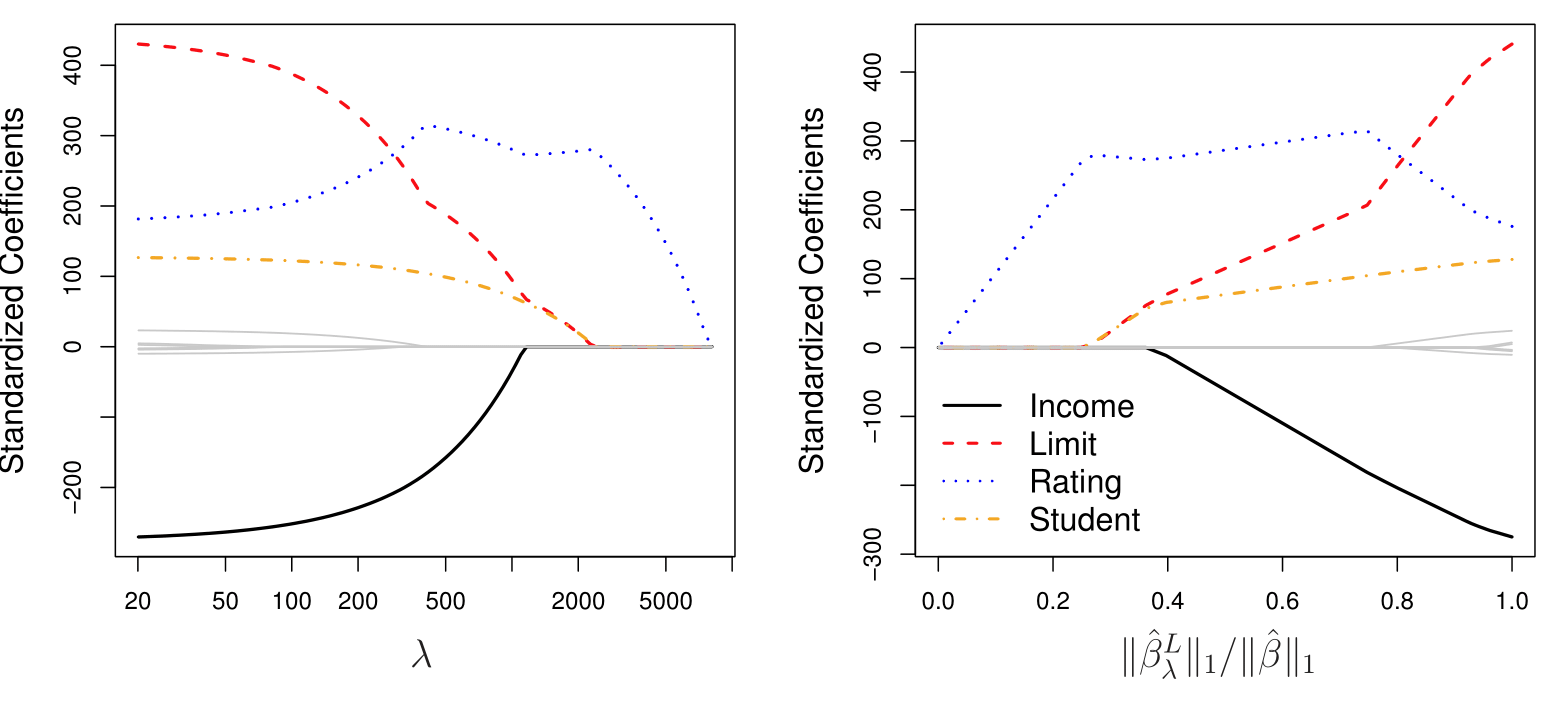
LASSO Coefficients

ILSR FIg 6.6: The standardized lasso coefficients on the Credit data set are shown as a function of \(\lambda\) and standardized \(\ell_2\) norm. Unlike least squares, ridge regression will produce a different set of coefficient estimates, \(\beta^R_\lambda\), for each value of \(\lambda\).

From left to right (in Right panel):

• 0 = null model (all 0 coefficients)
• first only rating
• then student and limit enter the model almost simultaneously,
• shortly followed by income.

Eventually, the remaining variables enter the model.

• Hence, depending on the value of λ, the lasso can produce a model involving any number of variables.
• In contrast, ridge regression will always include all of the variables in the model, although the magnitude of the coefficient estimates will depend on λ.

standardized coefficients (cuz we scaled)

ISLR simulation

A simulated data set containing \(p = 45\) predictors and \(n = 50\) observations.

ILSR 6.5 Squared bias (black), variance (green), and test mean squared error (purple) for the ridge regression predictions on a simulated data set, as a function of \(\lambda\) (left) and the standardize \(\ell_2\) norm (right). The horizontal dashed lines indicate the minimum possible MSE. The purple crosses indicate the models for which the MSE is smallest.

• \(\lambda < 10\) = 1e+01, the variance decreases rapidly, with very little increase in bias (hence MSE test drops considerably)
• \(\lambda\) = 0 = OLS, variance is high / bias low.

why right panel? - more comparable to the bias-trade off plots that we’re used to seeing. - From left to right: more flexible (bias decreases and the variance increases). - x-axis: coefficient estimates divided by the ℓ2 norm of the least squares estimates - these are the same pictures essentially but the y-axis on the RHS plotted against the $$2 norm of the ridge regression coefficient estimates divided by the $$2 norm of the least squares estimates.

Scaling of predictors

This property allows us to adjust the units or scale of predictors without changing the fundamental relationship modeled by the regression.

Least squares coefficients are scale equivariant

• i.e. multiplying \(X_j\) by a constant \(c\) leads to a scaling of the least squares coefficient estimates by a factor of \(1/c\).

In contrast, the ridge regression coefficient estimates can change substantially when multiplying a given predictor by a constant

• Why? since we use the sum of squared coefficients in the penalty term of the ridge regression objective function.

• If I multiply a feature by a constant it’s not going to matter because I can divide the coefficient by the same constant I get the same answer
• So it makes all the predictors comparable (and therefore their coefficients comperable)

Scaling of predictors (cont’d)

Therefore, it is best to apply ridge regression after standardizing the predictors, using the formula

\[\begin{equation} \tilde{x}_{ij} = \frac{x_{ij}}{\frac{1}{n} \sum_{i=1}^n (x_{ij} - \overline{x}_j)^2} \end{equation}\]

Note

Software will perform centering and standardizing by default and reports answers back on original scale.

• denominator: the estimated standard deviation of the jth predictor
• all of the standardized predictors will have a standard deviation of one

iClicker

iClicker: difference between Lasso and Ridge

What is the primary difference between LASSO and Ridge regression?

1. Ridge regression uses the L1 penalty while LASSO uses the L2 penalty.
2. Ridge regression can handle non-linear relationships, whereas LASSO cannot.
3. LASSO is used when the number of predictors is less than the number of observations, while Ridge is used when predictors exceed observations.
4. LASSO performs feature selection by setting some coefficients to zero, while Ridge only shrinks them. ✅ Correct

iClicker

iClicker: tuning paramter

In the context of LASSO and Ridge regression, what does the parameter \(\lambda\) control?

1. The intercept of the regression model

2. The degree of the polynomial in the model

3. The strength of regularization applied to the coefficients ✅ Correct

4. The number of predictors included in the model

Comment

• Unlike subset selection, which will generally select models that involve just a subset of the variables, ridge regression will include all predictors in the final model.
• In other words, \(\beta\) coefficients approach 0 but never are actually equal to zero.
• But adopting a small change on our penalty term, we will be able shrink coefficients exactly to zero (and hence perform feature selection) \(\dots\)

• RR is not able to perform feature selection
• Why is Ridge regression particularly useful in datasets with multicollinearity? It spreads the coefficient weight across correlated predictors, reducing the risk of large, unstable coefficients.

Benefits of LASSO

• It is worth repeating that the \(\ell_1\) penalty forces some of the coefficient estimates to be exactly equal to zero when the tuning parameter \(\lambda\) is sufficiently large

• Hence the lasso performs variable selection

• As a result, models generated from the lasso are generally much easier to interpret than those of ridge regression

• We say that the lasso yields “sparse” models — that is, sparse models that involve only a subset of the variables.

ex Benefit most: A high-dimensional dataset where only a few predictors are expected to be relevant

Benefits of Ridge Regression

• The lasso implicitly assumes that a number of the coefficients truly equal zero

• When this is not the case, i.e. all predictors are useful, Ridge Regression would leads to better prediction accuracy

• These two examples illustrate that neither ridge regression nor the lasso will universally dominate the other.

• The choice between Ridge Regression and LASSO can also boil down to the Prediction vs. Inference trade off (aka Accuracy-Interpretability trade off);

When to use what?

• One might expect the Lasso to perform better in a setting where a relatively small number of predictors have substantial coefficients, and the remaining predictors have coefficients that are very small or that equal zero

• Ridge regression will perform better when the response is a function of many predictors, all with coefficients of roughly equal size.

• Since we do not typically know this, a technique such as cross-validation can be used in order to determine which approach is better on a particular data set.

When to use Regularization

\(p > n\)

• These methods are most suitable when \(p > n\).

• Even when \(p < n\) these approaches (especially lasso) is popular with large data sets to fit a linear regression model and perform variable selection simultaneously.

• Being able to find, so-called “sparse” (as opposed to “dense”) models that select a small number of predictive variables in high-dimensional datasets is tremendously important/useful.

• variable selection is extremely important
• eg test for disease using 30K gene expressions (too expensive) so instead we find a test that works well on only 10 genes, that could be a major breakthrough
• much more meaningful for inference

When to use Regularization

Multicollinearity

• Less obviously, when you have multicollinearity¹ in your data, the least squares estimates have high variance.

• Furthermore, multicollinearity makes it difficult to distinguish which which variables (if any) are truly useful.

• Using the same argument as before, we can use ridge regression and lasso to reduce the variance and improve prediction accuracy and simultaneous shrink the coefficients of redundant predictors.

• by “useful” i mean predictive of the outcome.

• In the high-dimensional setting, the multicollinearity problem is a serious problem and makes it impossible to istinguish which which variables (if any) truly are predictive of the outcome

• At most, we can hope to assign large regression coefficients to variables that are correlated with the variables that truly are predictive of the outcome.

1. when two or more predictors in a regression are correlated with each other

Multicollinearity in Credit

pairs(Credit[,1:3])

• We can see that multicollinearity is an issue for the credit data for example.

• credit limit is highly related to credit rating

• and both or those are possitively correlated with income for example

iClicker

iClicker: which to choose

Why might you choose LASSO over Ridge regression?

1. When you want a model with non-zero coefficients for all predictors

2. When you want to reduce multicollinearity but retain all predictors

3. When the predictors are known to be independent of each other

4. When you want to perform feature selection and have some coefficients exactly equal to zero ✅ Correct

iClicker

iClicker

Which of the following statements is true about the bias-variance trade-off in LASSO and Ridge regression?

1. Increasing \(\lambda\) in both methods increases bias but decreases variance. ✅ Correct
2. Increasing \(\lambda\) in both methods decreases bias but increases variance.
3. Increasing \(\lambda\) in LASSO increases variance, while it decreases variance in Ridge.
4. LASSO increases bias, while Ridge increases variance.

Choosing \(\lambda\)

• Both the lasso and ridge regression require specification of \(\lambda\)

• In fact, for each value of \(\lambda\) we will see different coefficients.

• So how do we find the best one?

• The answer, as you may have guessed, is cross-validation.

similar to the \(\lambda\) parameter from our penalized MSE for pruning back trees

glmnet

To perform regression with regularization we use the function glmnet() function (from package glmnet )

glmnet(x, y, ... )

• Note that glmnet does not allow the formula argument¹.

• Hence we will need specify x and y.

• pronounced “glim - net”

1. N.B. there is a handy helper function model.matrix() that will help us do this.

glmnet penalty

glmnet(x, y, alpha = 1, ... )

The penalty used is: \[ \frac{(1-\alpha)}{2} || \beta ||_2^2 + \alpha ||\beta||_1 \]

• alpha=1 is the lasso penalty \(||\beta||_1\) (default)

• alpha=0 is the ridge penalty

Values between 0 and 1 are allowed and correspond to elasticnet (this model is not discuss here or in the book).

glmnet \(\lambda\)

glmnet(x, y, alpha = 1, nlambda = 100 ... )

• A grid of values for the regularization parameter \(\lambda\) is considered

• nlambda: the number of \(\lambda\) values considered in the grid (default=100)

• The actually values are determined by nlambda and lambda.min.ratio (see the help file for more on this)

• Alternatively, the user may supply a sequence for \(\lambda\) (in the optional lambda argument), but this is not recommended.

glmnet standardizing and family

glmnet(x, y, alpha = 1, nlambda = 100, standardize = TRUE,
  family = c("gaussian", "binomial", "poisson", "multinomial", 
             "cox", "mgaussian"), ... )

• By default the function standardizes the data¹

• The family argument specifies the distribution type for the response². We need family = "gaussian" for regression).

1. Coefficient estimates then transformed back onto original scale (by multiply back up by standard deviation) for the results.

2. Regularization can be extended to logistic and multinomial, and poisson regression. To learn more about family functions in R, run ?family in the R console

Cross-validation

• In order to determine the best choice for \(\lambda\) we use cross-validation

• The cv.glmnet function from the same package will perform \(k\)-fold cross-validation¹ for glmnet

• From that we produce a plot that returns good value(s) for \(\lambda\)

1. default is 10-fold

helper function

library(glmnet); library(ISLR2); data(Credit)
x <- model.matrix(Balance~., Credit)[,-1]
y <- Credit$Balance

• The model.matrix() function is particularly useful for creating x
• Not only does it produce a matrix corresponding to the predictors but it also automatically transforms any qualitative variables into dummy variables¹

• model.matrix is borrowed form the stats package
• [,-1] is to say we don’t need the intercept column (the intercept will still be fit but that is controlled within the function: glmnet(x, y, alpha = 1, intercept = FALSE))
• model.matrix(Balance~.-1, Credit) should do the same but some reason when you code it like that TWO dummy variables gets made for Own (yes/no)

1. this is important since glmnet() can only take numerical, quantitative inputs

Lasso with Credit

lasso <-  glmnet(x = x, y = y, family = "gaussian", alpha = 1)
plot(lasso, xvar = "lambda")

• Options for xvar are “norm”, “lambda”, “dev” (default is L1 norm)
• label = TRUE to label the curves
• ?plot.glmnet for details
• you can see how many non-zero variables are in the model on the “top”-axis

Lasso Coefficient Estimates

To see the values for the coefficient estimates use coef(). For example to the see coefficients produced when \(\lambda\) the 60th value in our sequence ( log \(\lambda\) = 0.4938434 in this case):

coef(lasso)[,60]

 (Intercept)       Income        Limit       Rating        Cards          Age 
-483.4397780   -7.5851123    0.1704558    1.3900860   15.4997658   -0.5597635 
   Education       OwnYes   StudentYes   MarriedYes  RegionSouth   RegionWest 
  -0.5160200   -6.8245847  418.6128482   -5.3459725    2.1876891    7.6654500 

Ridge Regression with Credit

note: 11 all the way across the top (we never loose predictors)

Cross-validation for RR

set.seed(10) # use cross-validation to choose the tuning parameter
cv.out.rr <- cv.glmnet(x, y, alpha = 0)
plot(cv.out.rr);  log(bestlam <- cv.out.rr$lambda.min)

[1] 3.680249

• the first (left-most) vertical dotted line is the best lambda (min)
• the second vertical dotted line is a second choice (the largest lambda that is within 1 standard error of the minimum)
• the second is a more restricted model that does almost as well (maybe even better) as the minimum
• 11 = at all stages we have all 11 predictors in our model

Cross-validation for Lasso

set.seed(1) # use cross-validation to choose the tuning parameter
cv.out.lasso <- cv.glmnet(x, y, alpha = 1)
plot(cv.out.lasso);  log(bestlam <- cv.out.lasso$lambda.min)

[1] -0.5295277

• similar plot for lasso.
  
• note the number of variables (11 - 6 = 5)

CV output plot

The cv.glmnet ouptut plot produced from a simulation that you will see in lab

This line is at lambda.1se, the largest λ value within one standard error of the minimum MSE.

It’s a slightly more conservative choice than lambda.min and often yields a simpler model by shrinking more coefficients.

It is typically preferred when there’s a desire for a more parsimonious model that may generalize better to new data.

Beer

beer.lm = lm(price~., data=beer[,-1]); summary(beer.lm)

...

Coefficients:
              Estimate Std. Error t value Pr(>|t|)    
(Intercept)  3.7174521  0.6807382   5.461 8.56e-07 ***
qlty        -0.0111435  0.0064446  -1.729   0.0887 .  
cal         -0.0055034  0.0089957  -0.612   0.5429    
alc          0.0764520  0.1752318   0.436   0.6641    
bitter       0.0677117  0.0153219   4.419 3.98e-05 ***
malty        0.0002832  0.0099639   0.028   0.9774    
---
Signif. codes:  0 '***' 0.001 '**' 0.01 '*' 0.05 '.' 0.1 ' ' 1

Residual standard error: 0.8661 on 63 degrees of freedom
Multiple R-squared:  0.6678,    Adjusted R-squared:  0.6415 
F-statistic: 25.33 on 5 and 63 DF,  p-value: 6.588e-14
...

Lasso on beer

lasso <-  glmnet( x = beer[,c(3:7)], y = beer[,2], family = "gaussian", alpha = 1)
plot(lasso, xvar = "lambda")

Best \(\lambda\) for LASSO

first column are names, second column is price

lambda.min minimizes the cross-validated MSE and gives the most accurate model on the validation set.

lambda.1se offers a simpler model within one standard error of the minimum error, providing a balance between model accuracy and complexity.

Lasso on beer

# superimpose the best lambda on trace plot
plot(lasso, xvar = "lambda")
abline(v = log(bestlam.lasso), col = "gray", lwd = 2, lty = 2)

Lasso on beer

library(plotmo) # allows us to label the x biggest coefs
plot_glmnet(lasso, xvar = "lambda", label = 5)
abline(v = log(bestlam.lasso), col = "gray", lwd = 2, lty = 2)

Lasso on beer

library(plotmo) # allows us to label the x biggest coefs
plot_glmnet(lasso, xvar = "lambda", label = 5)
lambda2 = cv.out.lasso$lambda.1se # 2nd choice 
abline(v = log(lambda2), col = "gray", lwd = 2, lty = 2)

Coefficients

cbind(coef(beer.lm),  # OLS (least squares estimates)
      # LASSO estimates ...
      coef(lasso, s = bestlam.lasso), # ... at best lambda
      coef(lasso, s = lambda2))       # ... at lambba within 1 s.e.

6 x 3 sparse Matrix of class "dgCMatrix"
                                    s1         s1
(Intercept)  3.7174521392  3.334440257 3.25063467
qlty        -0.0111434572 -0.008782345 .         
cal         -0.0055034319  .           .         
alc          0.0764519623  .           .         
bitter       0.0677117274  0.062008057 0.04831986
malty        0.0002831604  .           .         

Summary

• Ridge regression and LASSO works best in situations where the least squares estimates have high variance.

  • This can happen when \(p\) exceeds (or is close to \(n\))

  • It can also happen when we have multicollinearity

• LASSO shrinks coefficient estimates to exactly 0 hence it can be viewed as a variable selection technique

• Ridge Regression shrinks coefficient estimates close to 0 so it never actually eliminates any predictors.

Different Formulation

The coefficient estimates can be reformulated to solving the following two problems.

Lasso regression solve:

\[ \text{minimize} \quad \sum_{i=1}^{n} \left(y_i - \beta_0 - \sum_{j=1}^{p} \beta_j x_{ij}\right)^2 \quad \text{subject to} \quad \sum_{j=1}^{p} |\beta_j| \leq s \]

Ridge regression solves:

\[ \text{minimize} \quad \sum_{i=1}^{n} \left(y_i - \beta_0 - \sum_{j=1}^{p} \beta_j x_{ij}\right)^2 \quad \text{subject to} \quad \sum_{j=1}^{p} \beta_j^2 \leq s \]

• For every value of λ, there is some \(s\) such that the Equations RSS+λ\(\Sigma\)|βj| and (1) will give the same lasso coefficient estimate
• we’re trying to find the set of coefficient estimates that lead to the smallest RSS, subject to the constraint \(|\beta_j| \leq s\) (our budget)

Contours of the error and constraint functions for the lasso (left) and ridge regression (right). The solid blue areas are the constraint regions, \(|\beta_1| + |\beta_2| \leq s\) and \(\beta_1^2 + \beta_2^2 \leq s\), while the red ellipses are the contours of the RSS.

• OLS = \(\hat \beta\)
• Each of the ellipses centered around \(\hat \beta\) represents a contour: this means that all of the points on a particular ellipse have the same RSS value
• As the ellipses expand away from the least squares coefficient estimates, the RSS increases.
• circle = RR constraint
• diamond = LASSO constraint
• \(s\) makes those shapes bigger/smaller
• If \(s\) is sufficiently large, then the constraint regions will contain \(\hat \beta\), and the RR/LASSO estimates == OLS estimates
• When \(s\) gets smaller, the shapes get smaller at \(\hat \beta\) falls outside of diamond and circle (constraint region)
• The equations indicate that the RR/LASSO coefficient estimates are given by the first point at which an ellipse contacts the constraint region (circle/diamond).
• Since ridge regression has a circular constraint with no sharp points, this intersection will not generally occur on an axis, and so the ridge regression coefficient estimates will be exclusively non-zero.
• However, the lasso constraint has corners at each of the axes, and so the ellipse will often intersect the constraint region at an axis.
• In Figure 6.7, the intersection occurs at β1 = 0, and so the resulting model will only include β2.