Data 311: Machine Learning

Lecture 12: Boosting

Dr. Irene Vrbik

University of British Columbia Okanagan

Recap

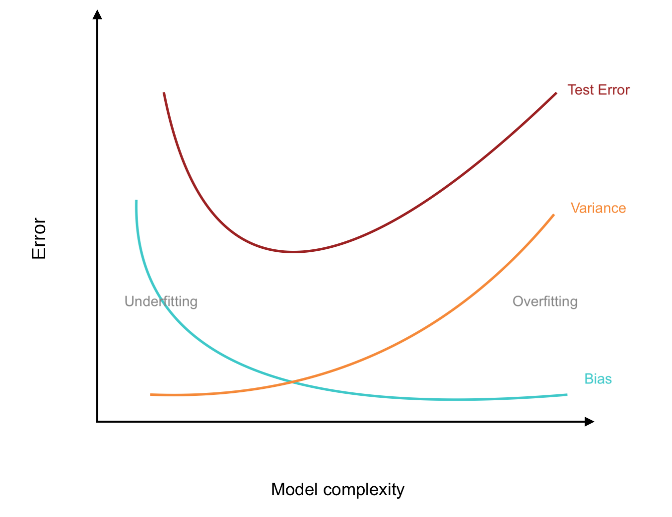
• Last time we saw how bootstrap aggregation (or bagging) can improve decision trees by reducing its variance.

• For Random Forest (RF) we use a similar method to bagging, however, we only consider m predictors at each split¹.

• That added randomness in RF further reduce the variance of the ML method, thus improving the performance even more.

• We now discuss boosting, yet another approach for improving the predictions resulting from a decision tree

1. for classification we usually use \(m = \sqrt{p}\) and for regression we use \(m = p/3\)

Preamble

• Again, we focus on decision trees, however, this is a general approach that can be used on many ML methods.

• Like bagging and RF, boosting involves aggregating a large number of decision trees; that is to say, it is another ensemble method.

• Unlike bagging and RF, boosting will combine the outcome of many trees to tackle bias.

Several supervised machine learning algorithms are based on a single predictive model,

• eg. linear regression,single decision trees, and support vector machines.

Bagging and random forests, on the other hand, work by combining multiple models together into an overall ensemble.

Since averaging reduces variance, bagging (and hence, random forests) are most effectively applied to models with low bias and high variance (e.g., an overgrown decision tree).

While boosting is a general algorithm for building an ensemble out of simpler models (typically decision trees), it is more effectively applied to models with high bias and low variance!

Although boosting, like bagging, can be applied to any type of model, it is often most effectively applied to decision trees (which we’ll assume from this point on).

Bushy Trees

bushy trees tend to overfit

Goal of Bagging

Bagging in starts with a model that overfits the data (CART)

and then we aggregate many models together to reduce the variance and bring the error and improve the performance

Stumps

boosting usually starts with a very simple model that tends to underfit the data, i.e. a model with high bias

one example of a simple model is a shallow tree (aka stump)

stumps tend to underfit

Goal of Boosting

boosting in a sequential procedure that “boosts” the model to make it more complicated boosting builds complex models out of simple ones to make it more complex and therefore reduce the bias

Summary: both attempt to reduce test error

• Boosting builds complex models out of simple ones to reduce bias
• Bagging average models to reduce variance (Commonly used with high-variance models like decision trees.

Boosting is a fairly simple variation on bagging that strives to improve the weak learners by focusing on areas where the system is not performing well.

From bagging to boosting

Some differences moving from bagging to boosting:

1. no more bootstrap sampling
2. trees are grown sequentially (as opposed to in parallel)
3. trees are added together rather than averaged.
4. rather than fitting “bushy” trees we prefer “stumps”

Bagging (Bootstrap Aggregating):

• Models are trained independently on different bootstrap samples of the dataset.

Boosting:

• Models are trained sequentially, with each new model focusing on correcting errors made by the previous ones.
• It aims to reduce both bias and variance by iteratively improving the model’s accuracy.
• Uses weighted data to prioritize difficult cases.

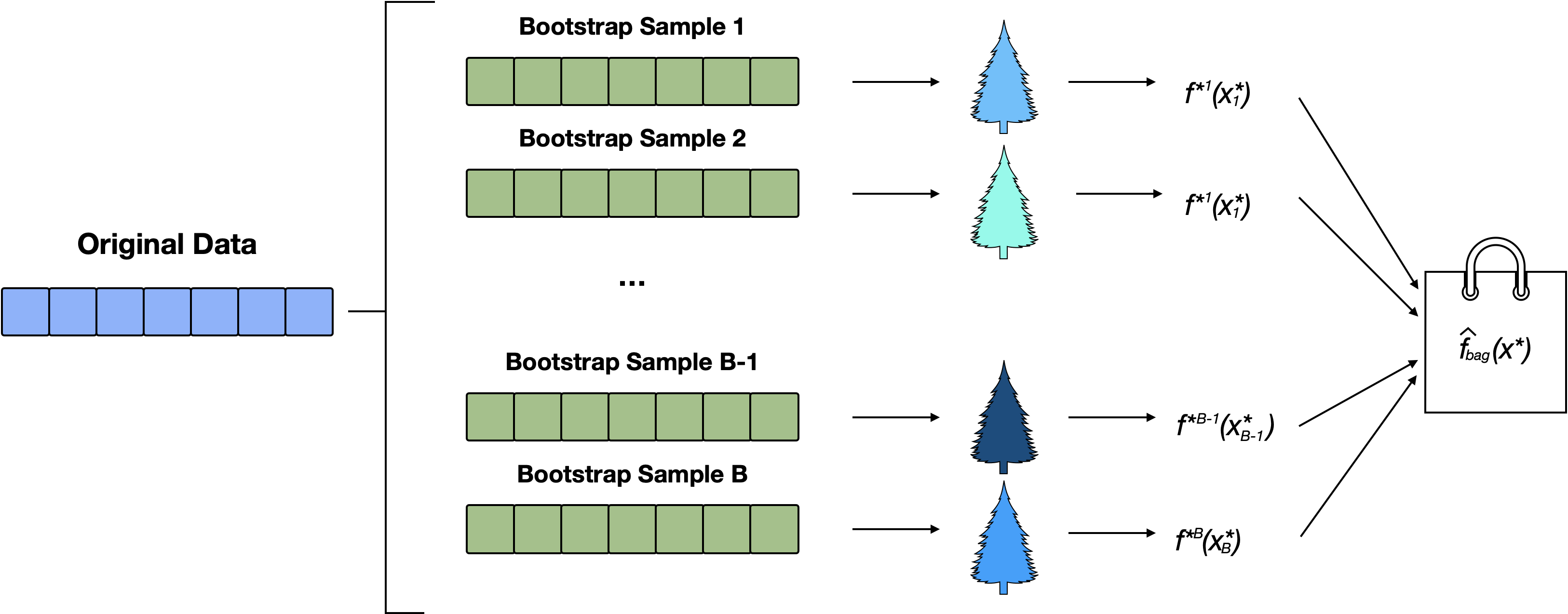
Bagging Schematic

Figure 1: Multiple (e.g. 500) bootstrap samples are sampled. Each sample is used to train an individual decision tree, resulting in a collection of diverse models. The predictions from all trees are then aggregated to produce a final, more robust prediction. This process reduces model variance and improves generalization compared to using a single tree.

• Bootstrap Sampling: Each decision tree is trained on a different bootstrap sample of the original dataset, which introduces variability among the trees.

• Feature Selection at Each Split: All features are considered when determining the best split at each node of the decision trees. This can lead to similar trees if some features are highly predictive.

• Diversity Source: The main source of diversity in bagging comes from the different bootstrap samples used to train each tree. However, the trees may still look quite similar if some features dominate the splits.

we get some variation due to the nature of bootstrapping, but the trees may look somewhat similar

N.B trees are grown independently on random samples of the observations. IOW, a random reshuffling of the bootstrap samples won’t make a difference since each tree is fitted in parallel

Random Forests

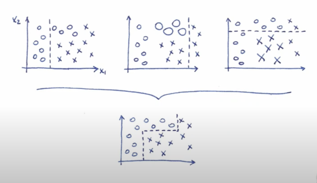
Random forest is an extension of bagging that randomly selects subsets of predictors at each split (thereby diversifying the forest even more than bagging).

Random forest is an extension of bagging that randomly selects subsets of predictors at each split (thereby diversifying the forest)

• Bootstrap Sampling: Like bagging, Random Forests also use bootstrap samples to train each tree, providing variability from different subsets of the data.

• Random Feature Selection at Each Split: At each split, a random subset of the features is considered (rather than all features). This introduces an additional layer of randomness, making the trees more diverse than in bagging.

• Diversity Source: The diversity in Random Forests comes from both the different bootstrap samples and the random feature selection at each split. This makes Random Forests generally better at reducing overfitting compared to bagging.

• average the predictions from these trees to reduce variance

• again these trees are fit in parallel

From Bushy Tree to Stumps

• Note that the bushy trees in RF (by design) may look quite different from one another (i.e. they will have difference decision rules, different sizes, etc…)

• In boosting, we make a forest of “short” trees (eg. \(d\)¹= 1, 4, 8, 32); maybe having one node and two leaves (aka stumps)

• These stumps are referred to as a “weak learners”²

• Weak Learner will be preferable to the boosting method which “learns slow” by additing these weak learnings together.

1. where \(d\) is the number of decision rules (see Boosting Tuning Parameters)

2. simple models that do only slightly better than random chance

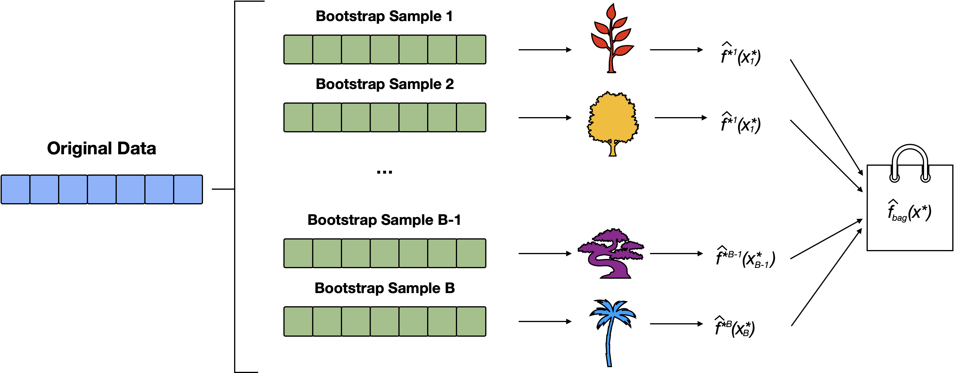
Boosting stumps

Figure 2: Boosting Stumps: Starting with the original data, boosting trains multiple ‘stumps’ (single-split decision trees). Note that these are NOT bootstrap samples and these trees are NOT trained in parallel.

Note: these are not bootstap samples

Note: these decesion trees are NOT trained in parallel!

Bootstrap is a sequential algorithm, whats different… what do each of these datasets look like if they’re not bootstrap samples

• Now: each tree is fit on a modified version of the original training data set.

Bye-bye bootstrap

• Boosting does not involve bootstrap sampling; instead each tree is fit to the residuals obtained from the last tree.

• That is, we fit a tree using the current residuals, rather than the outcome \(Y\), as the response.

• This approach will “attack” large residuals, i.e. will focus on areas where the system is not performing well.

Other key differences

• Trees will be grown sequentially such that each tree will be influenced by the tree grown directly before it.

• Like RF, boosting involves combing a larger number of decision trees \(\hat f_1, \dots, \hat f_B\), however…

• rather than taking the average (or majority vote) of the corresponding predicted values, the combined prediction is typically a weighted average (or a voting mechanism).

Apart from the bootstrap samples, there are other important differences between boosting and random forests:

• the weight is going to reflect how well that tree performed.
• learners that perform better are given more weight in the final prediction.

how do we bring these trees together?

How to ensemble

• By fitting small¹ trees to the residuals, we slowly improve \(\hat f\) in areas where it does not perform well.

• To slow this down even further, we multiple this fit by a small positive value set by our shrinkage parameter \(\lambda\).

• We add this shrunken decision tree into the fitted function to produce a small nudge in the right direction

• In general, statistical learning approaches that “learn slowly” tend to perform well.

• try to pick up a small piece of the signal with each subsequent tree

Empirical evidence shows that taking lots of small steps in the right direction results in better Predictions with a test set,

1. with just a few terminal nodes, determined by the parameter \(d\) in the algorithm.

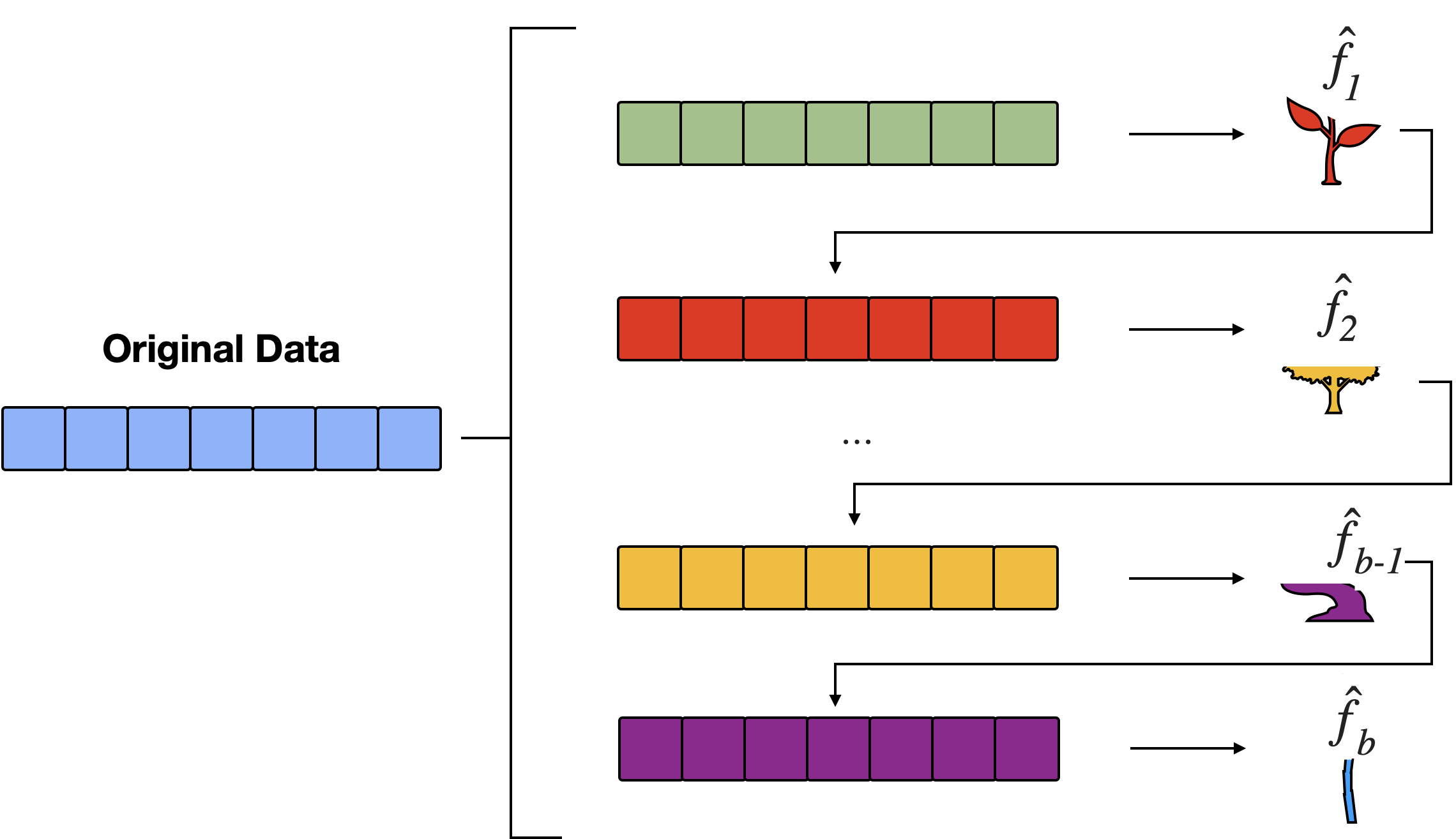
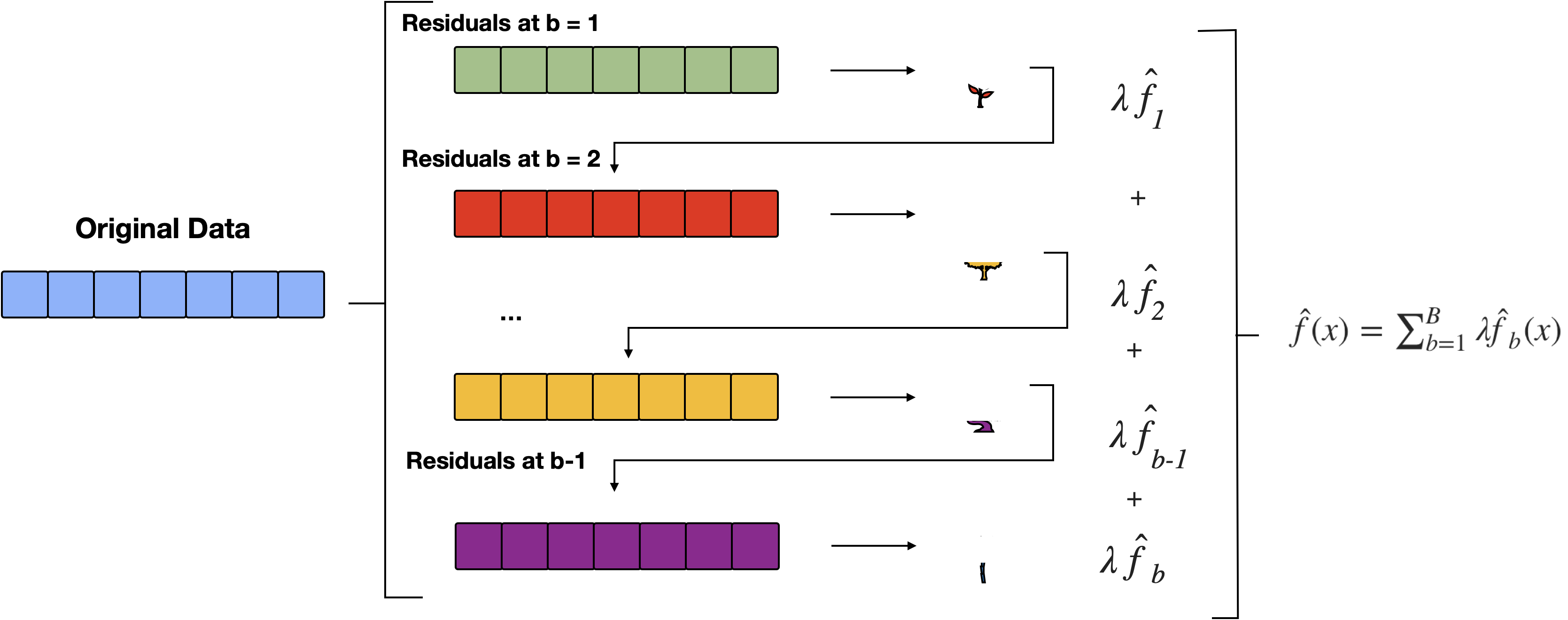
Boosting for Regression

Figure 3: Starting with the original data, the algorithm fits a sequence of simple models (stumps) to the residuals, aiming to correct errors from previous predictions. At each iteration, \(b\), the model predicts the residuals and updates the overall prediction by adding a scaled version of the current model’s output, weighted by the learning rate \(\lambda\). This iterative process continues for \(B\) rounds, producing the final boosted model as the sum of these weighted predictions, which gradually improves accuracy.

Algorithm

1. Set \(\hat f(x)=0\) and \(r_i =y_i\) for all \(i\) in the data set \((X, r)\).
2. For \(b= 1,\dots, B\), repeat:

   1. Fit a tree \(\hat f_b\) with \(d\) splits (\(d+1\) terminal nodes) to \((X,r)\)

   2. Add a shrunken version off this decision tree to your fit: \[\begin{equation} \hat f(x) = \hat f(x) + \lambda \hat f_b(x) \end{equation}\]

   3. Update residuals \(r_i = r_i - \lambda \hat f_b(x)\)

3. Output the boosted model \(\hat f(x) = \sum_{b=1}^B \lambda \hat f_b(x)\)

1. Start off with a short tree (maybe one decision node) on the original data

2.1. replace y with r and fit as normal (but don’t go all the way to bushy tree-stop when number of terminal notes is d+1) 2.2. so we shift our prediction slowly towards some direction

• we slowly improve \(\hat f\) in areas where it does not perform well.
• λ slows the process down, allowing more and different shaped trees to attack the residuals.
• notice how the tree relies on the outcomes of the previous tree
• no bootstrap sampling needed

Details on boosting for classification appears in Ch 10 of ESL (more complicated). Both problem can be handled with the gbm (gradient boosted model) package

Gene expression Data

Results from performing boosting and RF on the 15-class gene expression data set in order to predict cancer versus normal. The test error is displayed as a function of the number of trees. For the two boosted models, \(\lambda\) = 0.01. Depth-1 trees slightly outperform depth-2 trees, and both outperform the RF, although the standard errors are around 0.02, making none of these differences significant. The test error rate for a single tree is 24 %.

boosting can overfit (unlike bagging and rf), if

• iterations (number of trees) is too high or if t
• learning rate \(\lambda\) is set too large.

Since boosting adds models sequentially to reduce bias by focusing on the residuals (errors) of previous models, it can start fitting to the noise in the training data if continued for too long. However, using a smaller learning rate and applying early stopping (halting the boosting process when performance on a validation set stops improving) can help mitigate overfitting.

• A very simple model applied in a slow and sequential way with predict very well.
• typically one will try a few values of d (mabye 1,2,4, 8 )
• you can see a sort of leveling off which is typical in these classification problems,
• however it is possible to overfit if we set B too large
• so in some problems you could see this test error go up after a certain point, although it would take a really long time for that to happen.

Boosting Tuning Parameters

Boosting requires several tuning parameters:

• \(B\) = the number of fits (trees for today’s example)

  • Unlike bagging/RF, boosting can overfit if \(B\) is too large¹

• \(\lambda\) = learning rate for algorithm, a small positive number

  • e.g. 0.01 or 0.001 are common

• \(d\) = complexity or interaction depth (often \(d=1\) works well)

  • for trees, this is the number of rules (i.e. internal/decision nodes) so \(d+1\) is the number of terminal nodes.

• if the model is very simply \(\lambda\) will have to be pretty small (if the model is dumb it will take longer to learn) and need more trees
• if the model is more complex \(\lambda\) can be bigger and therefore learn quicker
• tune this using cross-validation
• Very small λ can require using a very large value of B in order to achieve good performance.

1. We could use cross-validation to select \(B\).

Benefits

• Improved Accuracy: By focusing on previously misclassified data points, boosting reduces bias and helps the model fit the training data more accurately.

• Reduced Overfitting: Boosting also reduces the risk of overfitting, as it combines the predictions of multiple weak learners, which helps generalize the model.

• Robustness: It can handle noisy data and outliers because it adapts to misclassified points.

• Unlike fitting a single large deci- sion tree to the data, which amounts to fitting the data hard and potentially overfitting, the boosting approach instead learns slowly.

iClicker

iClicker

How does boosting differ from bagging in terms of model training?

1. Boosting uses bootstrap samples, while bagging does not.
2. Bagging focuses on reducing bias, while boosting reduces variance.
3. Bagging requires a learning rate parameter, whereas boosting does not.
4. Boosting fits models sequentially, while bagging fits them in parallel.

iClicker

iClicker

Which statement is true about boosting?

1. It only reduces variance without affecting bias.
2. It trains models independently on different subsets of the data.
3. It can overfit if the number of iterations is too high.
4. It uses majority voting to combine predictions.

iClicker

iClicker

What type of base learner is typically used in boosting algorithms?

1. Complex (bushy) decision trees
2. Bagged trees
3. Simple models like stumps
4. Random forests

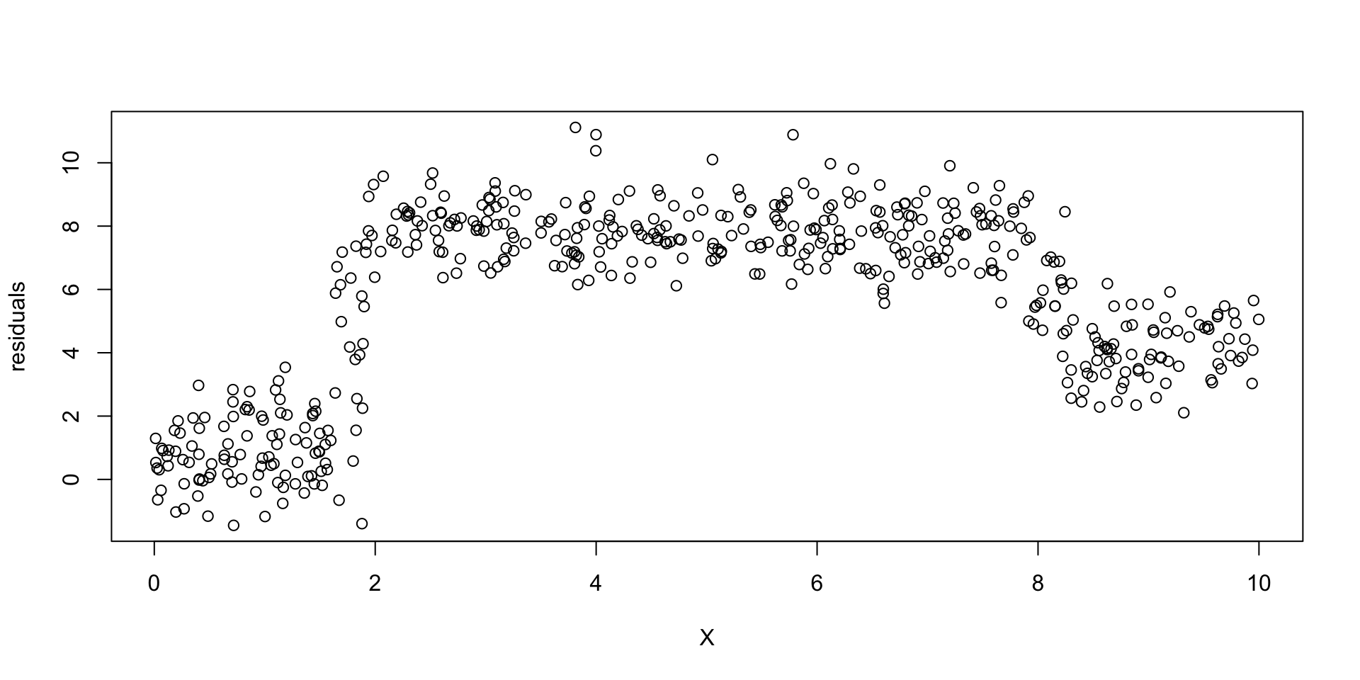
Example: Regression Simulation

Recall the regression simulation from our CART lecture:

head(dat)

Step 1:

Set \(\hat f(x)=0\) and \(r_i =y_i\) for all \(i\) in the data set \((X, y)\).

colnames(dat) <- c("X", "r"); round(dat,3)

Step 2a:

For \(b= 1,\dots, B\), fit a tree \(\hat f_b\) with \(d\) splits (\(d+1\) terminal nodes) to \((X,r)\)

fhat =  rep(0, nrow(dat))
lambda <- 0.005; B = 700; d = 1
for(i in 1:B){
  regt <- tree(r~X, data=dat, control=
                 tree.control(nobs = nrow(dat), mincut = 2, 
                    minsize = 4, mindev = 0.001))
  stump <- prune.tree(regt, best=d+1)
}

see ?tree.control():

• mincut = min obs to include in children nodes (default 5)
• minsize = smallest allowed node size (default 10)
• mindev = within-node deviance must be at least this times that of the root node for the node to be split (default = 0.01)

\(\hat f_1(x)\)

Step 2b:

… add a shrunken version off this decision tree to your fit:

fhat =  rep(0, nrow(dat))
lambda <- 0.005; B = 700; d = 1
for(i in 1:B){
  regt <- tree(r~X, data=dat, control=tree.control(nrow(dat), 2, 4, 0.001))
  stump <- prune.tree(regt, best=d+1)
  fhatb = predict(stump)
  fhat <- fhat + lambda*fhatb
  # ... more to do
}

\[\begin{equation} \hat f(x) = \hat f(x) + \lambda \ \hat f_b(x) \end{equation}\]

Shrunken Tree

\[ \begin{align} \hat f(x) &= 0 + \lambda \hat f_1(x)= \begin{cases} 0 + 0.005*1.355, \text{ if }<1.88734\\ 0 + 0.005*6.997, \text{ otherwise } \end{cases} \end{align} \]

Step 2c: update residuals

\[ \begin{align} r_{b} &= y - \hat f(x) \\ &= y - (0 + \lambda \ \hat f_1(x) + \lambda \ \hat f_2(x) + \dots + \lambda \ \hat f_b(x)) \\ &= r_{b-1} - \lambda \ \hat f_b(x) \end{align} \]

at \(b=0\) we have \(\hat f(x) =0\) and \(r_0 = y - \hat f(x) = y\)

\[ \begin{align} \text{at } b&= 1 & \text{at } b&= 2 \\ r_1 &= y - \hat f(x) & r_2 &= y - \hat f(x) \\ &= y - (\hat f_0(x) + \lambda \hat f_1(x)) & &= y - (\hat f_0(x) + \lambda \hat f_1(x) + \lambda \hat f_2(x)) \\ &= \underbrace{y - \hat f_0(x)}_{r_0} - \lambda \hat f_1(x) & &= \underbrace{y - \hat f_0(x) - \lambda \hat f_1(x)}_{r_1} - \lambda \hat f_2(x) \end{align} \]

fhat =  rep(0, nrow(dat))
lambda <- 0.005; B = 700; d = 1
for(i in 1:B){
  regt <- tree(r~X, data=dat, control=tree.control(nrow(dat), 2, 4, 0.001))
  stump <- prune.tree(regt, best=d+1)
  fhatb = predict(stump)
  fhat <- fhat + lambda*fhatb
  dat$r <- dat$r - lambda*fhatb
}

Plotted residuals

Now we fit a tree to this dataset.

this might look the same but it’s actually the residuals

Algorithm Visualization

Top right: current stump:

Bottom right: summed model \(\hat f(x) = \hat f(x) + \lambda \hat f_b(x)\)

Main ideas:

• Learns slowly (this is every 10th iteration)
• starts by attacking that high residual that big jump that corresponded to our root node in our original regression tree (thats going to be the case for a while)
• at each iteration we’re trying to pick up a little piece of the signal
• no given tree on its own is going to do a good job

Algorithm Comments

• Given the current model, we fit a decision tree to the residuals (each tree relies on the previous tree)
• We then add a shrunken version of this decision tree to the fitted function \(\hat f\) (to nudge it a bit in the right direction)
• Each tree can be rather small (determined by \(d\))¹

By fitting small trees to the residuals, we slowly improve \(\hat f\) in areas where it does not perform well.

1. \(d\) = 1 in our case, i.e. 2 terminal nodes

Step 3

Output the boosted model \(\hat f(x) = \sum_{b=1}^{860} \lambda \hat f_b(x)\)

• this crashes sometimes (code in lab)
• actually goes much slower as this is showing every 10th tree
• this additions can be negataive
• 700 trees plots every 10

Boosting Resources

• Boosting for classification is similar in spirit to boosting for regression, but it is a bit more complex

• ISLR2 does not going into the details but you can find them in Elements of Statistical Learning, Chapter 10

• To perform boosting with trees (both in the classification and regression setting), we can use the gbm() (_Gradient Boosted Models) function from the gbm package.

Boosting for Classification

Boosting repeatedly applies a weak binary classifier \(G : \mathbb{R}^p \rightarrow \{-1, 1\}\) to the training set, modifying sample weights:

• Start with equal sample weights \(w_i = 1/n\).
• For steps \(m = 1, \ldots, M\):
  • Fit a classifier \(G_m\) to the training data using weights \(w_i\).
  • Compute its weight \(\alpha_m\) given its performance.
  • Update the sample weights \(w_i\) to increase the importance of misclassified samples.
• Output \(G(x) = \text{sign}\left(\sum_m \alpha_m G_m(x)\right)\).

the choice of \(\alpha_m\) (the weight for each classifier) and the update of sample weights \(w_i\) depend on the classifier’s performance.

ESL Figure 10.1: Schematic of AdaBoost. Classifiers are trained on weighted versions of the dataset, and then combined to produce a final prediction.

Boosting Example

Source: https://www.youtube.com/watch?v=thR9ncsyMBE&t=1980s&ab_channel=T%C3%BCbingenMachineLearning

1. performs not very well but better than chance.
2. The circles that are misclassified gets bigger weights so the algorithm is forced to focus on them. the result tree stump is different
3. We increase the weight of the misclassified crosses,

… keep going. This will never coverge. you will keep getting more models.

The decision boundary gets more and more complicated the more you boost.

Most popular is ada boost - how we choose the \(\alpha\) and weights.

Boosting function

library(gbm)
gbm(formula, distribution = "bernoulli", n.trees = 100,
  interaction.depth = 1, shrinkage = 0.1)

• distribution = “bernoulli” (for binary 0-1 responses), “gaussian” (for regression), “multinomial” for multi-class

Tuning parameters:

• interaction.depth = \(d\),
• shrinkage = \(\lambda\)
• n.trees = \(B\).

You can overfit here, so play around with these

Comments about gbm

While the gbm() function is used for boosting in the textbook, note that when you do boosting for a multi-class classification problem you will get the following warning:

Setting distribution = "multinomial" is ill-advised as it is currently broken. It exists only for backwards compatibility. Use at your own risk.

• XGBoost is known for its computational efficiency
• highly optimized, making it faster and more scalable compared to GBM
• However it uses Regularization: XGBoost includes L1 (Lasso) and L2 (Ridge) which makes it less interpretible

Other package options exist (eg. tree booster in Extreme Gradient Boosting xgboost instead)

Example: Sine Function

A simulation where x has a true underlying sine wave relationship (blue line) with y along with some irreducible error.

fit using gmb

library(gbm)

# Fit a gradient boosting model with decision stumps
boost_model <- gbm(y ~ x, data = dat, 
                   distribution = "gaussian", # aka regression
                   n.trees = 1000, 
                   interaction.depth = 1, 
                   shrinkage = 0.01)

Tuning parameters:

• interaction.depth = \(d = 1\),
• shrinkage = \(\lambda = 0.01\)
• n.trees = \(B = 1000\)

Plot at different stages

Example: Wine

Let’s perform boosting on the wine data set from the gclus package. As this is a multi-class classification problem, be advised that running this will produce a warning.

library(gbm)
library(gclus); data(wine)
weak.lrn <- gbm(factor(Class)~., distribution="multinomial",
              data=wine, n.trees=5000,
              interaction.depth=1)

Example: Wine

To get a sense of the test error and compare with bagging and RF, we can again use a cross-validation approach (here LOOCV)

library(gbm)
library(gclus); data(wine)
cvboost <- NA
for(i in 1:nrow(wine)){
  # preform boosting on the cross-validation training set
  weak.lrn <- gbm(factor(Class)~., distribution="multinomial",
                data=wine[-i,], n.trees=5000,
                interaction.depth=1)
  # Prob x_i belongs to the g = 1, 2, 3 group
  pig = predict(weak.lrn, n.trees=5000,
                newdata=wine[i,], type="response")
  # predict the class for the ith validation observation
  cvboost[i] <- which.max(pig) 
 }

• takes some time to run
• I had to cache the results from this chunk

CV error rate

   cvboost
     1  2  3
  1 58  1  0
  2  1 70  0
  3  0  0 48

This cross validated error rate is 1.12%. In this case boosting is equivalent to RF in terms of prediction. Recall:

RF (1.12%) > Bagging (3.37%) > Simple Tree (8.43%).

very good results for this data

Example: body

Recall the body data from the gclus pacakge:

• It contains 21 body dimension measurements as well as age, weight, height, and gender on 507 individuals;

• so \(p = 24\) (treating gender as our binary response)

1. Fit boosting using the validation approach (train/test) to obtain est of err
2. Fit RF and obtain the OOB error est
3. Compare est of eff from train/test (3.29) with cross-validated (1.38)

body: Boosting

set.seed(45613)
library(gbm); data(body) # code doesn't work is Gender is factor
train <- sample(1:nrow(body), round(0.7*nrow(body)))
bodyboost <- gbm(Gender~., distribution="bernoulli", data=body[train,],
                n.trees=5000, interaction.depth=1)
pprobs <- predict(bodyboost, newdata=body[-train, ], type="response",
                  n.trees=5000) 
(boosttab <-  table(body$Gender[-train], pprobs>0.5 ))

   
    FALSE TRUE
  0    74    0
  1     5   73

Test misclassification rate is 3.29%

Let’s use gbm to apply boosting to the body data with 5000 trees, with trees up to depth 1

• validation approach is subject to a lot of variabiliy so lets do cv
• improvement will level out; see last example ISLR lab

body: Random Forests

set.seed(4521)
library(randomForest)
(bodyRF <- randomForest(factor(Gender)~., data=body, importance=TRUE))

Call:
 randomForest(formula = factor(Gender) ~ ., data = body, importance = TRUE) 
               Type of random forest: classification
                     Number of trees: 500
No. of variables tried at each split: 4

        OOB estimate of  error rate: 3.94%
Confusion matrix:
    0   1 class.error
0 251   9  0.03461538
1  11 236  0.04453441

• class.error = 9/(251+9) = 0.0346154
• class.error = 11/(236+11) = 0.0445344

Boosting with cross-validation

# be patient in lab, code will take some time to run
load("data/boostbodyCV.RData")
(tab <- table(body$Gender, as.numeric(cvboost)))

   
      0   1
  0 257   3
  1   4 243

Misclassification rate as estimated by CV is 1.38%

Example: beer

• Consider the beer data analyzed in previous lectures.

• Using beer price as our outcome, the cross validated boosting RSS is 97.9 (i.e. its worst of the options we’ve tried)

• Notable the training RSS is 3.86 (code omitted - see lab)

What is this an indication of?

• Ans: that boosting is overfitting to the beer data.

• i don’t want to undersell but i don’t want to over sell
• As a cautionary tale, realize that we can overfit with boosting.
  
• we didn’t play around with the tuning parameters too much so i’m sure we can do better

Variable Important measure

• In bagging and RF we saw how we got a measure of Variable Importance which essentially ranks the predictors.

  • In regression we record the total amount that the RSS is decreased due to splits over a given predictor, averaged over all \(B\) trees.
  • In classification, we add up the total among that the Gini index is decreased by splits over a given predictor, averaged over all \(B\) trees.

• A large value indicates an important predictor

• Similar measures/plots are calculated in boosting

Beer: Variable Importance Table

summary(beerboost)

Beer: Variable Importance Plot

summary(beerboost)

Boosting Comments

• Boosted models are incredibly powerful.

“best off-the-shelf classifier in the world” - Leo Breiman

• Generally speaking we have this relationship:

\[\text{Single Tree} < \text{Bagging} < \text{RF} < \text{Boosting}\]

• often win Kaggle competitions in predictive modelling for example ans: cross-validation
• Using smaller trees can aid in interpretability as well; for instance, using stumps leads to an additive model.

Tuning suggestions

• If learning rate \(\lambda\) is small then number of trees (\(B\)) and/or tree complexity (\(d\)) needs to increase.

• Tree complexity has approximate inverse relationship with the learning rate. AKA, if you double complexity, halve the learning rate and keep the number of trees constant.

• At least 1000 trees when dealing with small sample sizes (eg, \(n\) = 250) is recommended.

The easiest answer, is through cross-validation. But a complete grid-search becomes problematic with three parameters, so…

Summary

• Decision trees are simple and interpretable models for regression and classification
• However, they are often not competitive with other methods in terms of prediction accuracy
• Bagging, RF and boosting are good ensemble methods for improving the prediction accuracy of trees.
• The later two methods – RF and boosting – are among the state-of-the-art methods for supervised learning; however, their results can be difficult to interpret.

emsemble methods - wors by frowing many trees and aggregating them