Data 311: Machine Learning

Lecture 11: Bootstrap Aggregating (Bagging) and Random Forests

Dr. Irene Vrbik

University of British Columbia Okanagan

Introduction

Trees have one aspect that prevents them from being ideal tool for predictive learning, namely inaccuracy. - ESL

• We’ve just wrapped up some discussion on decisions trees, or CARTs which suggests that they are not particularly “good” models in many scenarios.

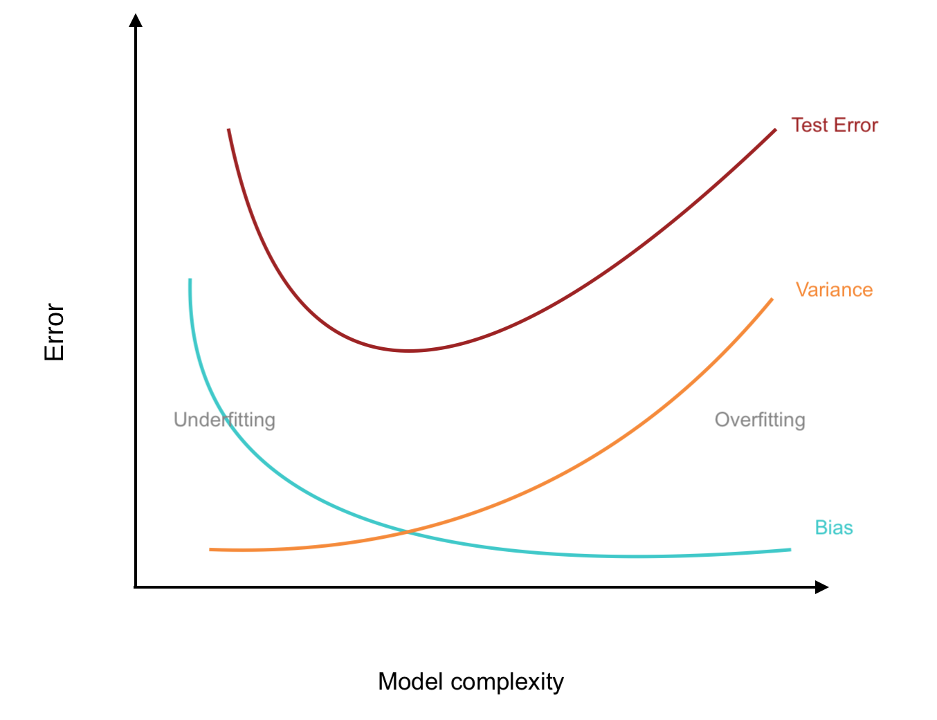
• Why? Bushy trees tend to have high variance and pruned trees have high bias

• Cons: don’t do very well in prediction: why?bushy tree had high variance pruned trees have high bias
• Pros: Easy to interpret

Preface

Today we’ll be looking at some ensemble methods to make them more competitive:

Namely, we will be looking at two embsemble methods:

• Bagging, which combines multiple models trained on random subsets to reduce variance

• Boosting which sequentially builds models that correct previous errors to reduce bias

“Two heads are better than one only if they contain different opinions” - Kenneth Kaye (January 24, 1946 – May 26, 2021[1]) was an American psychologist and writer whose research, books, and articles connect the fields of human development, family relationships and conflict resolution.

• Trees are easy to build, easy to use, and easy to interpret.

We’ll look at some ensemble methods to make them more competitve

This lecture correspondes to ISLR Chapter 8.2.1, 8.2.2, 8.2.3. More details can see: Random Forests with R by Robin Genuer, Jean-Michel Poggi (2020) available at UBC library

Preface

Namely, we will be looking at two embsemble methods:

• Bagging, which combines multiple models trained on random subsets to reduce variance

  • We’ll also look at Random forests, a specific type of bagging technique with an additional layer of randomness to improve model performance.

• Boosting which sequentially builds models that correct previous errors to reduce bias (covered next lecture)

Bushy Trees

bushy trees tend to overfit

Goal of Bagging

Bagging in starts with a model that overfits the data (CART)

and then we aggregate many models together to reduce the variance and bring the error and improve the performance

Stumps

boosting usually starts with a very simple model that tends to underfit the data, i.e. a model with high bias

one example of a simple model is a shallow tree (aka stump)

stumps tend to underfit

Goal of Boosting

boosting in a sequential procedure that “boosts” the model to make it more complicated boosting builds complex models out of simple ones to make it more complex and therefore reduce the bias

Summary: both attempt to reduce test error

• Boosting builds complex models out of simple ones to reduce bias
• Bagging average models to reduce variance

Ensemble Methods

Ensemble methods are techniques that combine the predictions of multiple models to improve overall predictive performance. Then can be divided in two groups:

1. Parallel Learners: multiple models are trained independently of each other.
   • e.g. Bootstrap Aggregation (Bagging), Random Forests
2. Sequential learners: models are trained sequentially, one after another. Each model in the sequence is typically trained to correct the errors made by the previous models.
   • e.g. Boosting, AdaBoost, Gradient Boosting, XGBoost

The idea behind ensemble methods is that by combining the strengths of different models, the ensemble can often outperform individual models and provide more accurate and robust predictions. Some common ensemble methods include:

• AdaBoost is a popular boosting technique that assigns more weight to misclassified observations, so subsequent models pay more attention to those challenging cases.

• Gradient Boosting is another sequential method where new models are added to minimize the loss function of the entire ensemble, effectively correcting the residual errors from the previous iteration.

• XGBoost is an optimized version of Gradient Boosting, known for its speed and efficiency.

• By aggregating the output of several models, ensemble methods can reduce overfitting, increase predictive performance, and improve generalization compared to using a single model.

Bagging

• Bagging (Bootstrap Aggregating) combines multiple models trained on different bootstrap samples (random subsets with replacement) to reduce variance.

• Because CART models tend to overfit the training data, we will use bagging to combine multiple “bushy” trees.

• This approach creates a more robust and generalizable model with lower variance than any single CART model.

While bagging is a general method used to reduce variance in high-variance algorithms by combining many models that are individually trained on slightly different subsets of data.

• CART models tend to overfit the training data, especially when the tree is allowed to grow deep, i.e. “bushy trees”.

• Bagging is used to improve performance by reducing their variance and making them more stable.

Why? Think of independent observations \(X_1, …, X_n\) having variance \(\sigma^2\); Central Limit Theorem tells us that their average value, i.e. \(\overline{X}\) will have variance \(\frac{\sigma^2}{n} (<\sigma^2)\)

General bagging

1. Generating \(B\) bootstrapped samples

2. Train \(B\) models, \(\hat f^{*b}\) for \(b = 1, \dots B\),

3. Aggregate the predictions

For regression this is simply the average prediction:

\[ \begin{equation} \hat f_{bag}(x) = \frac{\sum_{b=1}^B f^{*b}(x^*_b)}{B} \end{equation} \]

• Bagging method introduced by Breiman (1996)
• Recall a bootstrap sample is a sample of size n with replacement
• instead of just using the bootstrap models to estimate SE, we use them in our predictions (average each one to obtain one prediction)
• averaging a set of observations reduces variance: why? think of iid \(Xi\)s; \(\overline X\) will have less variance (\(\sigma^2/n\)) than \(X_i\) (\(\sigma^2\)).
• for each bootstrap sample we build a tree, and find \(\hat f^{*b}\) we average those values (or majority vote for classification)
• Bagging (or bootstrap-aggregating) can be thought of as applying the bootstrap to an entire model-fitting process, rather than just to estimate standard errors of estimators.

for classification we use a majority voting

What does it do: Combines multiple models (e.g., decision trees) trained on different bootstrap samples to reduce variance.

Why It’s Needed: High-variance models like deep decision trees (CART) often overfit the data.

How It Works:

1. Train models on different bootstrap samples (with replacement).

2. Aggregate predictions to improve stability:

   • Average for regression.
   • Majority vote for classification.

Result: Produces a more robust and generalizable model by smoothing out individual model errors.

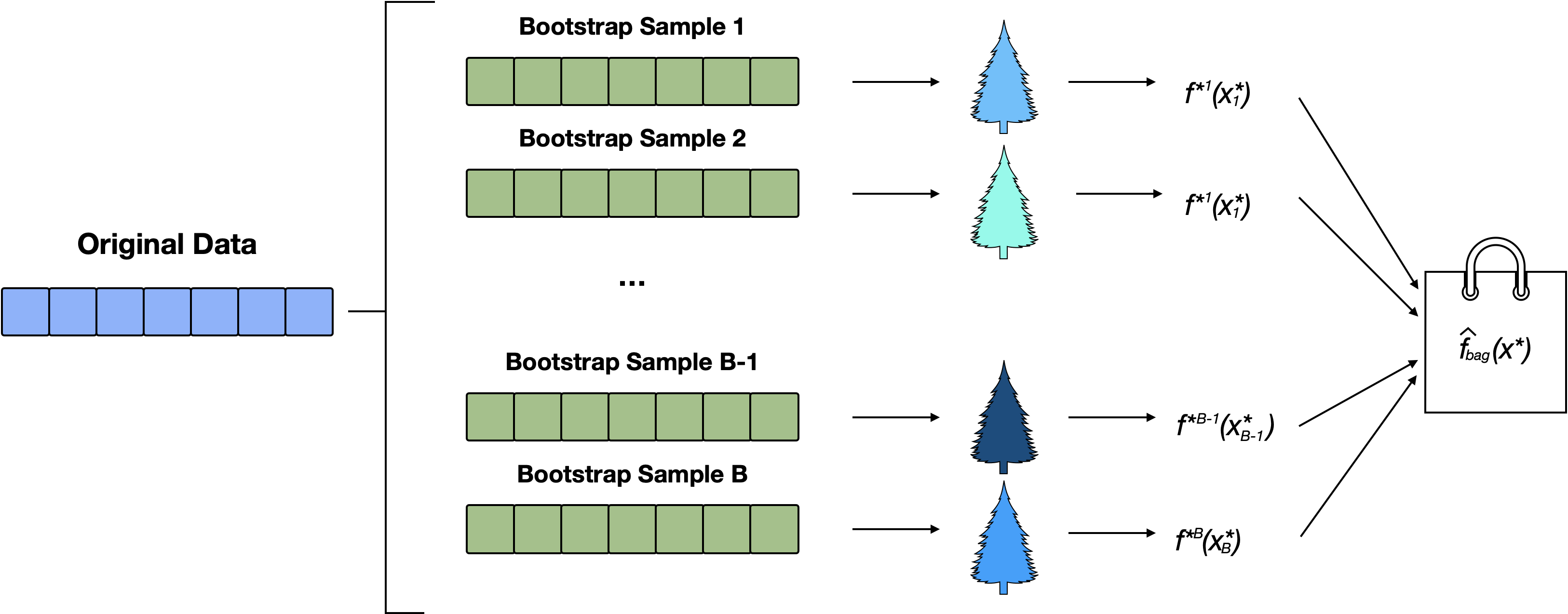
The main idea is to pool a collection of random decision trees

Source for image

1. Create B Bootstrap samples (sample with replacement of size \(n\))
2. Fit a (bushy) tree to each one
3. Each decision tree is used to make predictions
4. Aggregate the predictions (for regression the individual tree predictions are typically averaged, for classification we use a majority vote).

KEY: Using a bootstrap sample and considering only a subset of variables at each step results in a wide variety of trees. The variety is what makes random forests more effective than individual decision trees

Comments

• These trees for each bootstrap sample are grown deep (i.e. “bushy”), and are not pruned.

• Consequently, each individual tree will have high variance, but low bias

• The textbook suggests \(B=100\) as generally sufficient, but probably 500 to 1000 is safer (500 is the default).

• there is no need for pruning anymore cuz averaging will take care of that for us
• we use an average of trees to improve their prediction error
• 2 heads are better than one..
• simple models are the “building block”
• no harm in using more since we can’t overfit

Bagging Schematic

Figure 1: Bagging is an ensemble algorithm that fits multiple trees on different bootstrap samples, then combines the predictions from all models in a single bagged prediction.

1. Bootstrap Sampling: Multiple subsets of the training data are generated by randomly sampling the original dataset with replacement. Each subset is known as a bootstrap sample, and it may contain duplicates of some data points while missing others.

2. Independent Model Training: Each bootstrap sample is used to train an independent version of the model. Because each model sees a different variation of the dataset, the resulting models are diverse and may produce different predictions.

3. Aggregation of Predictions: After all the models are trained, aggregation is used to combine their predictions:

   • For regression tasks, the final prediction is the average of all the individual model predictions.

   • For classification tasks, the final prediction is determined by majority voting—the class that receives the most votes across all the models is chosen as the final output.

Compare with RF Schematic

Model Assessment

We could get an estimate of error using our test set, however, we can get a different estimate “for free”:

• Recall: a bootstrap sample consists of sampling \(n\) observations with replacement from our training set¹

• As we are sampling with replacement, some observations are randomly left out while others are duplicated.

• It can be shown that for each bootstrap sample, on average roughly \(\frac{1}{3}\) of the observations will not appear …

How do we know if our model is any good?

• We could get an estimate of error using the validation approach or CV, however, will help us estimate error

1. where \(n\) is the number of samples in our training set

Probability calculations

\[ \Pr(x_i \text{ is not selected in the bootstrap sample}) \]

\[ \begin{align} = P(x_i & \text{ is not selected on first draw}) \times \dots \\ & \quad \dots \times P(x_i \text{ is not selected on $n^{th}$ draw}) \end{align} \]

\[ \begin{align} &= \left(\frac{n-1}{n}\right)\times \dots \times \left(\frac{n-1}{n}\right) = \left(1 - \frac{1}{n}\right)^n \\ \end{align} \]

Now if we take the limit as \(n \to \infty\) we get:

\[ \begin{equation} \lim_{n \to \infty} \left(1 - \frac{1}{n}\right)^n = \frac{1}{e} \approx \frac{1}{2.7183} \approx \frac{1}{3} \end{equation} \] where \(e\) is the exponential constant approximately 2.718

Bootstrap Visualization

Image source: rasbt.github

The figure above illustrates how three random bootstrap samples drawn from an ten-sample dataset \((x_1,x_2,...,x_{10})\) and their ‘out-of-bag’ sample for testing may look like.

• In the first bootstrap sample, \(x_3, x_7, x_{10}\) are not selected
• In the second bootstrap sample, \(x_6, x_9\) are not selected
• In the third bootstrap sample, \(x_3, x_7, x_8, x_{10}\) are not selected

OOB observations

• The observations not included in the bootstrap sample during bagging are called the Out of Bag (OOB) observations.

• These OOB observations can serve a similar role as the validation sets in cross-validation

• By serving as internal validation, OOB provides an efficient way to evaluate model performance, making it a practical alternative to cross-validation.

Another advantage of bagging is that it provides an internal estimate of predictive performance, which closely aligns with cross-validation or test set estimates.

• OOB can think as out of the Bootstrap
• our training set for cv will be the other 2/3 (0.666*n)
• Consequently, we can estimate things like test error “for free”.
• This leads us to an interesting option for bootstrap-aggregated models…

Recall 5-fold CV Visualization

Similarities - training and testing/validation sets

Differences - in CV fold training set \(<n\) (\(= n - n/k\)) whereas bootstrap training set is size \(n\) - in CV each observation appears exactly one in the validation sets whereas in bootstrap, the can appear in multiple validation sets - in bootstrap the same observation may appear multiple times in a given trainging set

Consequently, we can estimate things like test error “for free”.

Aggregating OOB Predictions

For each training observation \(x_i\)​, predictions are made using only the models where \(x_i\)​ was an OOB observation¹.

• For regression, the OOB prediction for \(x_i\) is the average predictions from the OOB models:

  \[ \hat{y}_i^{\text{OOB}} = \frac{1}{B_i} \sum_{b \in \text{OOB}i} \hat{y}_{i}^{(b)} \]

• For classification, the OOB prediction is determined by majority voting among the models for which \(x_i\) was OOB.

• Each model is trained on a bootstrap sample that contains roughly two-thirds of the training observations (this leaves about one-third of OOB observations)

1. Let \(B_i\) represent the number of models where \(x_i\) was OOB, which, on average, is approximately \(B/3\)

OOB Error Estimation

For regression we calculate the Mean Squared Error (MSE): \[ \text{OOB MSE} = \frac{1}{n} \sum_{i=1}^{n} (y_i - \hat{y}_i^{^\text{OOB}})^2 \] where \(y_i\) is the true value and \(\hat{y}_i^{\text{OOB}}\) is the OOB prediction for observation \(x_i\). For classification we calculate the misclassification rate: \[ \text{OOB Error} = \frac{1}{n} \sum_{i=1}^{n} I(y_i \neq \hat{y}_i^{\text{OOB}}) \]

After obtaining OOB predictions for all training observations, the overall OOB error can be computed:

• bagging is fairly robust to overfitting (since it is already averaging across many varied model fits)
• alternatively we can use MSE but RSS is easier to access sometimes
• We can measure how accurate our RF is for a classification as the proportion of out-of-bag samples that were correctly

where \(I()\) is an indicator function that equals 1 if the true label \(y_i\) differs from the predicted label \(\hat{y}_i^{\text{OOB}}\), and 0 otherwise.

So if we wanted to predict the response for \(x_3\) we would use the trees fitted to Bootstrap sample 1 and Bootstrap sample 3 and average the result.

Key Points:

• OOB observations are those that are not included in the bootstrap sample used for training each model.
• OOB error provides an internal validation estimate of the test error, similar to cross-validation but without explicitly creating validation sets.
• The OOB estimate is efficient and a reliable alternative to cross-validation, particularly for large datasets.

iClicker

Number of Bootstrap observations

On average, what proportion of the training dataset is included in each bootstrap sample used to create the training set in bagging?

1. roughly 1/3

2. roughly 2/3 ✅ Correct

3. roughly \(n\), the number of samples in the training set

4. exactly, \(n\), the number of samples in the training set

iClicker

Purpose of bagging

What is the main purpose of bagging in ensemble methods?

1. To increase bias

2. To reduce variance ✅ Correct

3. To increase overfitting

4. To improve interpretability

iClicker

OOB observations

What is the main purpose of using the bootstrap in the context of bagging?

1. To create varied samples of the training data ✅ Correct

2. For estimating the test error without needing a separate validation set

3. To make the model deterministic

4. For feature selection

Example: Beer

Recall the beer data from last lecture (names removed):

69 observations and 7 columns

An example of six decision trees independently trained on bootstrap samples of the beer dataset. Each tree is slightly different due to the unique bootstrap sample used for training. This variability helps reduce model variance when predictions are aggregated across all (e.g. 500) trees. Compare with random forests

Illustrates Diversity Each tree is slightly different because the training data varied due to random sampling with replacement, which introduces diversity into the model training process. This variability reflects how bagging reduces overfitting by incorporating diverse perspectives from multiple models, which helps smooth out noise in the data.

Aggregating Predictions Reduces Variance: When the predictions from all these individual trees are aggregated (e.g., by averaging for regression or majority voting for classification), it results in a more stable and generalizable model. The ensemble will have lower variance than any individual tree, making the final prediction more reliable.

Remember, there are 500 of these

Notice how malty is the root decision for the 6th tree

Example: Beer OLS Regression

OLS Regression:

beerdat <- beerdat[,-1] 
attach(beerdat)
# linear model
beerlm <- lm(price~., data=beerdat)

Regression tree

library(tree);  par(mar=c(0,0,0,0))
beert <- tree(price~., data = beerdat) 
plot(beert)
text(beert, digits=4)

for a means of comparison we’ll fit a Ordinary Least squares regression model…

Rather than using the training - testing (validation procedure) were going to do cross-validation since this data set is so small (69 data points)

• First rule: BITTER, Second rule: BITTER, Third rule: BITTER
• we see bitter, qlty, bitter, cal, malty but we don’t see alcohol
• notably bitter seems to be a pretty important predictor

Cross-validation Errors

library(DAAG)
beercv<-cv.lm(data=beerdat, beerlm, m=10,printit=FALSE)

Let’s calculate the CV RSS error for OLS Regression:

# Get the CV estimate of MSE (two ways)
rss_lm = sum((beercv$price-beercv$cvpred)^2) # 10-fold CV RSS for lm
cv_mse <- attr(beercv, "ms") 
cv_mse*nrow(beerdat) # same as rss_lm above

[1] 57.33652

and the (actual) CV RSS error estimate for Regression Trees…

library(tree); set.seed(456); 
cv.beert <- cv.tree(beert); 
#10-fold CV RSS for 6 terminal tree
min(cv.beert$dev) 

[1] 77.56593

• so the linear model is a better model
• now lets get the OOB estimate

Bagging Regression Trees in R

library(randomForest); set.seed(134891)
p = 5 # number of predictors to consider at each split
(beerbag <- randomForest(price~., data=beerdat, ntree=500, mtry = p)) 

...
               Type of random forest: regression
                     Number of trees: 500
No. of variables tried at each split: 5

          Mean of squared residuals: 0.9338468
                    % Var explained: 54.71
...

We’ll talk in more detail of the code in second, but this is how we do a bagged model of 500 classification trees.

To get the OOB RSS, we multiple the OOB MSE estimate by \(n\), the size of our training set:

\[ \begin{align} MSE &= RSS/n \implies RSS = MSE \times n = 0.93 \times 69 = 64.44. \end{align} \]

Comparison

We can see that bagging has an improvement over the single tree, but not over OLS regression.

Model price~.	Estimate of Error (RSS)
Linear model	57.34 (from CV)
(Single) Regression Tree	77.57 (from CV)
(500) Bagged Regression Trees	64.44 (from OOB)

• ntree = 500 is the default
• mtry = p, the number of predictors
• foreshadow: random forest is to come
• %var explained (like a \(R^2\))

Error Comments

• It’s worth noting that comparison we just made…

• Technically, we have not performed cross validation on our bagged trees, and yet we are comparing the (OOB) error to properly cross-validated errors for LM and CART

• OOB estimation is a similar (and more efficient) way for providing realistic long term error estimates

• Takeaway: For practical purposes, OOB error from bagged models can be compared to CV error from other models.

Variable Importance

• The ensemble of trees helps identify which variables are most influential in the model.
• Another thing we get “for free” in bagging decision tress is a measure of variable importance.
• To quantify variable importance, we measure how much each variable improves the model’s predictions.

For bagging regression trees we focus on (RSS), while for bagging classification trees we focus on the Gini index.

Variable Importance in R

• We can obtain an overall summary of the importance of each predictor if requested using:

beer2 <- randomForest(price~., data=beerdat, ntree=500, 
      mtry = 5, importance = TRUE)

• Two measures are provided for variable “importance”¹.

• The plot and values are produced using the following:

varImpPlot(beer2)   # plot
importance(beer2)   # values (not shown in slides)

1. the two measure may not agree

Bagging Variable Importance Plots

Jump to RF varImpPlot

• as expected, bitter is imporant, and alcohol content is not important
• note there is a difference in ordering between cal and qlty
• for both the higher the better

%IncMSE (Percent Increase in Mean Squared Error): how much the MSE increases when the values of a given predictor are randomly permuted (while others remain the same).

IncNodePurity (Increase in Node Purity): measures the total improvement in splitting criteria (RSS for regression trees) when the variable is used for splitting.

Key Differences:

• %IncMSE focuses on prediction accuracy, showing how much worse the model performs without each variable.

• IncNodePurity focuses on split quality, indicating how much each variable improves the homogeneity of the target variable in the resulting splits.

Together, these measures provide complementary insights into which predictors are most important for the model. %IncMSE is often preferred for understanding variable importance in predictive performance, while IncNodePurity offers insights into the structural role of variables in the decision trees.

%IncMSE

1. Calculate the OOB MSE for the full set of \(B\) trees in your random forest, say, \(\text{MSE}_{full}\)

2. For the variable in question, randomly shuffle the observations (leave the order correct for the other columns).

3. Carry out predictions, calculate \(\text{MSE}_{shuff}\) then check the change from the full version for the variable in question: \[\begin{align} \text{%IncMSE} = \frac{\text{MSE}_{{shuff}}-\text{MSE}_{full}}{\text{MSE}_{full}} \end{align}\]

For classification we’ll measure the average increase in misclassification error when variables are randomly permuted.

• when I shuffle on that predictor, does it increase my MSE?
• If a predictors is not imporant (eg alcohol) shuffling it shouldn’t make a huge difference in MSE, so in the numerator you get something close to 0.
• If the variable is very important shuffling its values will lead to a noticeable increase in MSE, indicating that the model’s predictions rely heavily on that predictor.
• can extend to misclassication %IncMSE is simply the average increase in squared residuals of the test set when variables are randomly permuted (little importance = little change in model when variable is removed or added)

Higher values \(\implies\) variable is more important. For classification, MeanDecreaseAccuracy is used in place of %IncMSE

IncNodePurity

• IncNodePurity is the total increase in node purity obtained from splitting on the variable, averaged over all trees.

• In other words, IncNodePurity is the increase in homogeneity in the data partitions.

• For regression, “purity” is measured by residual sum of squares (RSS)¹.

• A higher increase of node purity indicates that the variable is more important.

• the documentation isn’t great for these measures so i wouldn’t get so bogged down in the details on how they are calculated
• takeaway is that bigger is better

1. For classification, we use the Gini index, so MeanDecreaseGini is used in place of IncNodePurity.

Bagging vs Single Tree

Cons

❌ We no longer have one model, but an average of many models!

❌ Bagging looses the interpretability of our model

❌ It is comparatively slower than fitting a single tree

Pros

✅ Averaging prevents overfiting

✅ improves prediction

✅ OOB error estimate “for free”

✅ Variable importance “for free”

✅ Doesn’t require CV/test set

• no more flowchart, more like a black box
• varaible importance - A large value indicates an important predictor
• Bagging improves prediction accuracy at the expense of interpretability.

Random forests

• Random Forests (RF) improve upon bagging by introducing a small tweak that decorrelates the trees.

• Like bagging, RF build a number of trees on bootstrapped training samples; however, each time a split in a tree is considered, a random sample of \(m\) predictors (where \(m < p\) = the total number of predictors) is considered.

• The default for classification is \(m = \sqrt{p}\) where \(p\) is number of predictors, and for regression \(m = p/3\)

• get it? “forests” have many trees

• “random” because a random sample of \(m\) predictors are considered at each split

• ()

• During tree growth for all \(B\) samples, at each split a number of the predictors is randomly removed from consideration

• In other words, in building a random forest, at each split in the tree, the algorithm is not even allowed to consider a majority of the available predictors.

• This decreases the dependency (or correlation) across the \(B\) trees, decreasing the variance of the averaged model (think back to LOOCV) and therefore increasing stability.

• As with bagging, we still loose interpretability over simple trees, but still gain the variable importance measure.

• Bagging is a special case of random forests when \(m = p\)

• LOOCV has higher variance than k-fold because there’s a lot of correlational among the model fits

• random forest makes a more diverse ecosystem

• “Since individual trees are randomly perturbed, the forest benefits from a more extensive exploration of the space of all possible tree predictors, which, in practice, results in better predictive performance”. (random forests with r book)

• small m will typically be helpful when we have a large number of correlated predictors.

First introduced by Leo Breiman in 2001 [paper]

RF Schematic

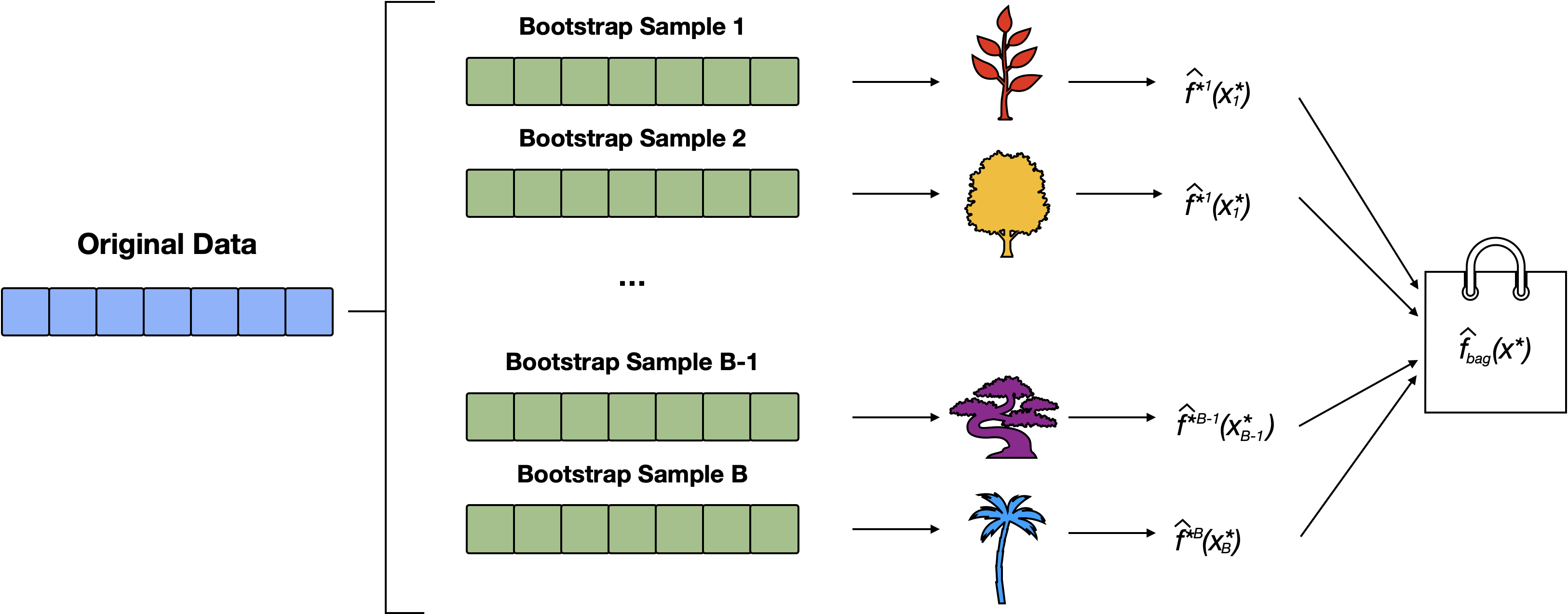
RF build on bagging by training multiple trees on different bootstrap samples and adding an extra layer of randomness by selecting a random subset of features at each split. This approach results in more diverse trees and better model generalization. Compare with Bagging Schematic

Both RF and Bagging start with \(B\) bootstraped samples

Feature Selection at Each Split: 

• Bagging considers all \(p\) predictors at each split

• At each split, a random subset of the features is considered (rather than all features). This introduces an additional layer of randomness, making the trees more diverse than in bagging.

Diversity Source:

• Bagging: different bootstrap samples used to train each tree. However, the trees may still look quite similar if some features dominate the splits.

• RF: from both the different bootstrap samples and the random feature selection at each split. This makes Random Forests generally better at reducing overfitting compared to bagging.

Motivating example

• Suppose that there is one very strong predictor in the data set (eg. bitter in the beer example)

• In the collection of bagged trees, most or all of the trees will likely use this strong predictor in the top split, hence, all of the bagged trees will look quite similar to each other.

• As discussed in our CV lecture, averaging highly correlated models does not lead to as large of a reduction in variance as averaging many uncorrelated quantities.

• decorelates the trees: Tropical forests rather than tundra biome
• During tree growth for all \(B\) samples, at each split a number of the predictors is randomly removed from consideration
• “The general idea of this method is that the random perturbation on individuals, brought by bootstrap sample draws, is not sufficient to promote diversity among trees and that it is also necessary to perturb the construction of trees at the variable level.” (RF with R book)

An example of six decision trees independently trained on bootstrap samples of the beer dataset in a RF. Each tree is different due to the unique bootstrap sample and the random selection of features at each split. This variability helps reduce model variance when predictions are aggregated across all (e.g., 500) trees. Compare with bagging

Steps for RF

1. Create \(B\) bootstrap samples

2. Fit a tree* to each bootstrap sample,

   * when creating nodes in each decision tree, only a random subset of \(m\) features is considered for splitting at each node.

3. Each decision tree is used to make a prediction.

4. Aggregate the \(B\) predictions.

*helps to decorrelate the trees

The default for classification is \(m = \sqrt{p}\) where \(p\) is number of predictors, and for regression \(m = p/3\)

R function

We use the randomForest() function from the randomForest package to implement bagging and RF. Usage:

randomForest(formula, ntree=500, mtry, importance=FALSE)

• ntree: the number of trees to grow (default = 500)
• mtry: the number of variables randomly selected at each node (default in classification is \(\sqrt{p}\) and \(p/3\) in regression; where \(p\) is the number of predictors).
• importance Should importance of predictors be assessed?

• ntree should not be set to too small a number, to ensure that every input row gets predicted at least a few times.

Optimizing the RF

• How do we determine how many subsets of features to consider at each split?

• mtry is a hyperparameter of our model and it’s choice can impact the performance of our random forest.

• In practice the default values are reasonable starting point and often works well in practice.

Alternatively you could use cross-validation to choose; e.g. build a random forest with mtry = \(\sqrt{p}-5\), \(\sqrt{p}\), \(\sqrt{p}+5\) and select the RF with highest accuracy

Random Forest on beer

mtry = \(\sqrt{p}\) by default¹

(beerRF <- randomForest(price~., mtry = sqrt(5), # default
            data=beerdat, importance=TRUE))

...
               Type of random forest: regression
                     Number of trees: 500
No. of variables tried at each split: 2

          Mean of squared residuals: 0.8469584
                    % Var explained: 58.93
...

The OOB estimate for RSS = MSE\(\times n\) = 0.847 * 69 = 58.44

\(\sqrt{5} = 2.236068\)

1. actually its floor(sqrt(p)) (which rounds down to the nearest integer).

Comparison

Method	RSS Estimate
Linear model	57.34
Random Forest	58.44
Bagging	64.44
Single Tree	77.57

For the beer data set, RF does better than single tree and bagging; however, it does still not outperform our linear regression model.

general simple Tree < Bagged tree < RF

RF Variable Importance Plot

Jump to Bagging varImpPlot

• notice how the ordering is not the same
• same pros and cons as bagging however RF is improved version of bagging

iClicker

RF vs bagging

In Random Forests, what additional step is taken compared to bagging to further reduce overfitting?

1. Training on larger dataset

2. Averaging the results of multiple models

3. Randomly selecting a subset of features at each split ✅ Correct

4. Using a single tree for predictions

iClicker

OOB error

What does the term “Out-of-Bag (OOB)” error refer to in the context of Random Forests and Bagging?

1. Error on a separate test dataset

2. Error on the original training set

3. Error calculated on the samples not used in the bootstrap sample ✅ Correct

4. Error on a validation dataset

Classification Example

• The smaller (more common) Italian red wine data set

• 178 samples of wine from three varietals (Barolo, Barbera, Grignolino) grown in the Piedmont region of Italy with 13 chemical measurements, i.e. \(p=13\)

• Let’s compare a single classification tree to a tree found using bagging and random forests …

library(gclus); data(wine); n = nrow(wine)

pretty good separation on Favanoids and Pehnols

pretty good separation on intensity

Single Decision Tree

winetree <- tree(factor(Class)~., data=wine)
plot(winetree); text(winetree)

• splits that are non-sense (same class predictions with splits)
• by-product of growing trees with Gini

Cost-complexity pruning

Pruned Classification Tree

Cross-validation error estimate

Let’s obtain the test error (in this case misclassification rate) by cross-validation at the minimum value of \(\alpha\):

# Find the index of the minimum cross-validated deviance in 'winetreecv'
min.idx <- which.min(winetreecv$dev)

# minimum CV deviance (total number of misclassified obs)
(miscl.obs <- winetreecv$dev[min.idx])

[1] 15

# Calculate the misclassification rate
(mscr <- miscl.obs / n)

[1] 0.08426966

The CV misclassification rate estimate is 15/178 \(\implies\) 8.43%

• pretty good for such a simple model!
• k-means only misclassifies 6 of the 178 wines 3.37%
• whereas HC misclassifies 29 of them 16.29%

Single pruned tree results

not bad but can bagging improve it?

Bagging wine

library(randomForest); set.seed(41351); 
winebag <- randomForest(factor(Class)~., mtry=13, 
                        data=wine, importance=TRUE)

• Here we are saying we want to do bagging mtry = \(m = p\)

• The importance argument tells the aglorithm that we want it to compute variable importance.

Note that now, we don’t have a single tree which we can plot.

Bagging Results

winebag

Call:
 randomForest(formula = factor(Class) ~ ., data = wine, mtry = 13,      importance = TRUE) 
               Type of random forest: classification
                     Number of trees: 500
No. of variables tried at each split: 13

        OOB estimate of  error rate: 3.37%
Confusion matrix:
   1  2  3 class.error
1 57  2  0  0.03389831
2  1 68  2  0.04225352
3  0  1 47  0.02083333

The OOB error rate of 3.37% versus 8.427% for a standard tree

• 2/(57+2) = 0.0338983
• (1+2)/( 1 +68 +2) 0.0422535
• 1/(47+1) 0.0208333

• this is an OOB confusion matrix (majority vote)

Bagging varImpPlot wine

Jump to RF varImpPlot

Random Forests

# use default: mtry = floor(sqrt(p)) = floor(sqrt(13)) = floor(3.605551)
(wineRF <- randomForest(factor(Class)~.,  # ntree = 500,
              data=wine, importance=TRUE))

...
                     Number of trees: 500
No. of variables tried at each split: 3
        OOB estimate of  error rate: 1.12%
Confusion matrix:
   1  2  3 class.error
1 59  0  0  0.00000000
2  1 69  1  0.02816901
3  0  0 48  0.00000000
...

\(\quad\) Simple Tree (8.43%) < Bagging (3.37%) < RF (1.12%)

sqrt(13) = 3.605551

RF varImpPlot wine

Jump to bagging varImpPlot

Summary of RF

• Random forests share many of the same pros and cons as Bagging vs Single Tree.

• They are considered one of the best “off-the-shelf” machine learning models due to their strong predictive performance.

• Random forests require minimal hyperparameter tuning (mainly the number of features to consider at each split, mtry or \(m\)), and the default settings usually perform well in most cases.