Data 311: Machine Learning

Lecture 9: Bootstrap

Dr. Irene Vrbik

University of British Columbia Okanagan

Introduction

• Last lecture we saw a resampling method called cross-validation (CV) for estimating test error.

• Now, a resampling method called the bootstrap where we repeatedly sample from a dataset with replacement.

• This allows us to estimate the distribution of a statistic (such as a standard deviation) when we only have limited data.

• Hence, it can quantify the uncertainty associated with a given estimator¹ or statistical learning method.

Relates to ideas from STAT 230. We don’t just want a point estimate for \(\mu\) say, we rather want a confidence interval.

1. An “estimator” or “point estimate” is a statistic (that is, a function of the data) that is used to infer the value of an unknown parameter in a statistical model.

Motivation

• Sometimes it is possible to work out things like bias and standard error (SE) of an estimator in closed form.

• For example the standard error of \(\overline X\), the estimator for the mean of a normally distributed population with having (unknown population) mean \(\mu\) and variance \(\sigma\), is \[\text{SE}(\overline X) = \frac{\sigma}{\sqrt{n}}\]

Sampling Distribution of \(\overline X\)

More specifically if \(X_i\) are i.i.d¹ Normal(\(\mu\), \(\sigma^2\)), then \(\overline X=\frac{1}{n}\sum_{i=1}^n X_i\) has the sampling distribution given by:

\[ \overline X \sim \text{Normal}(\mu, \frac{\sigma}{\sqrt{n}}) \]

Recall that the standard error of an estimator simply refers to the standard deviation of the sampling distribution of that estimator.

1. independent, identically distributed

Motivation (cont’d)

From this information we could create 95% confidence intervals for our estimate of \(\mu\)

\[ \begin{equation} \bar{x}\ \pm \ t_{0.025, n-1} \left(s/\sqrt{n}\right) \end{equation} \]

• \(\bar{x}\) is the sample mean.
• \(t_{\frac{\alpha}{2}, \, n-1}\) is the critical value from the \(t\)-distribution with \(n-1\) degrees of freedom
• \(s\) is the sample standard deviation.
• \(n\) is the sample size.

Sampling Distribution

• Generally speaking a sampling distribution is the probability distribution of a statistic (or estimator) that is obtained through repeated sampling of a specific population.

• In simulations, we could generate large number of samples and record the value of the statistic of interest to obtain an empirical estimate of the sampling distribution.

• In many contexts, only one sample is observed, but the sampling distribution can be found theoretically.

Question: “How can we estimate the reliability of a machine learning model using a single (small) dataset?”

• If an arbitrarily large number of samples were separately used in order to compute one value of a statistic, then the sampling distribution is the probability distribution of the values that the statistic takes on.

• sampling distributions are incredibly important in statistics because they allows us to do inference. eg. obtain confidence intervals and conduct hypothesis test

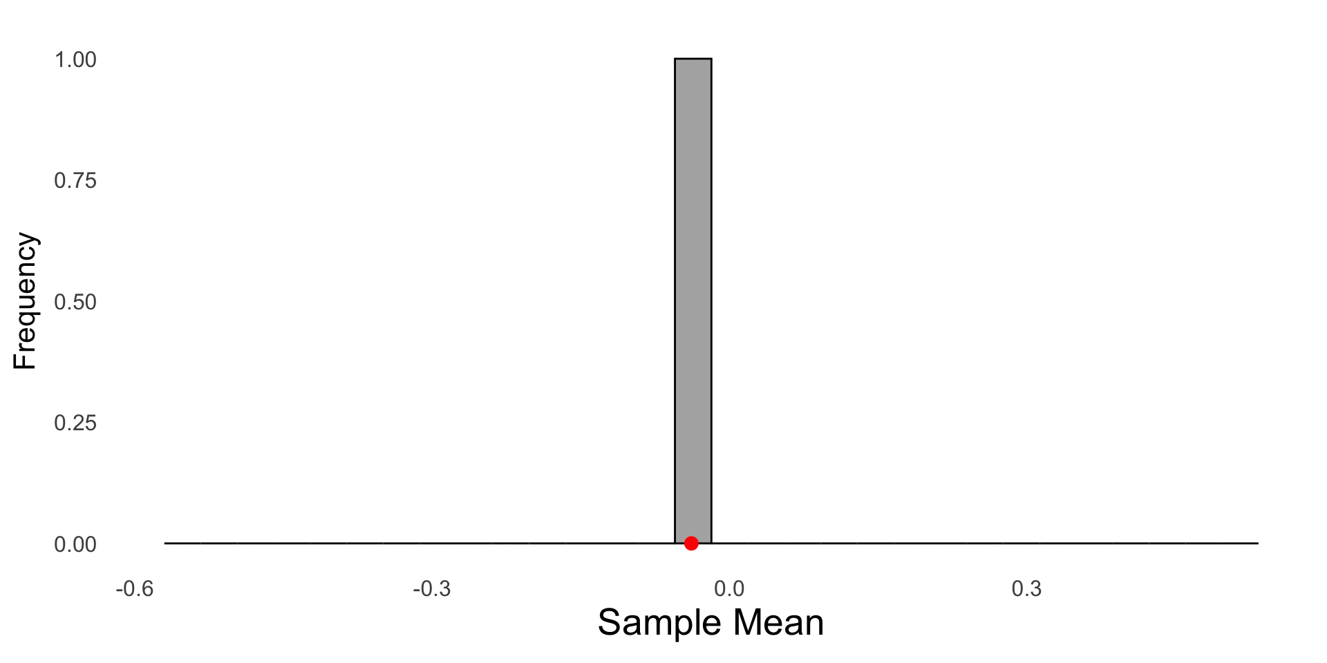
The sample mean from 1000 random samples drawn from a standard normal N(0,1) are saved and plotted in a histogram. Each red dot represents the sample mean of a random sample of size 30 from the population.

The Sampling Distribution gives us a sense of how \(\bar{X}\) might change from sample to sample.

• there is a high likelihood we’d get something close to the original mean (0)
• and getting something relatively “far” from \(\mu\), e.g. -0.6, should be relatively rare.

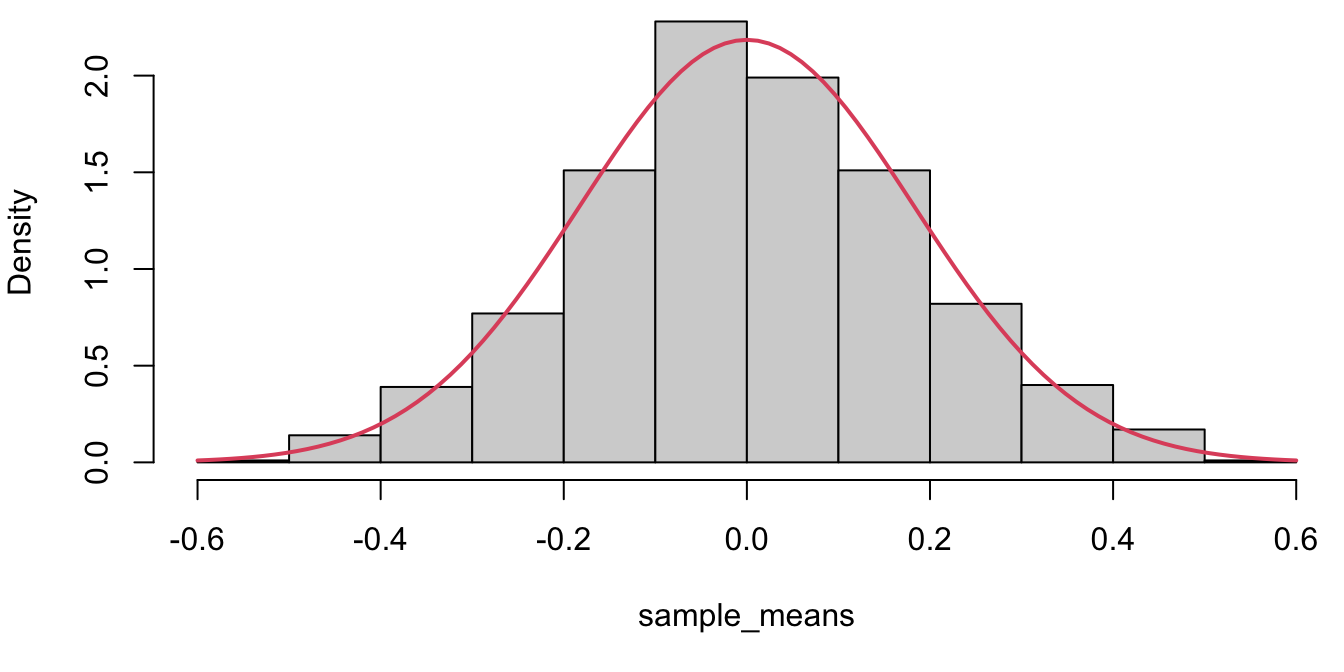
Simulated vs Theoretical

A histogram of 1000 sample means; each \(\bar{X}\) was calculated from a (different) random sample of size 30 drawn from a N(0,1) population. The red curve represents the theoretical sampling distribution of \(\bar{X} \sim N(0, 1/\sqrt{30})\)

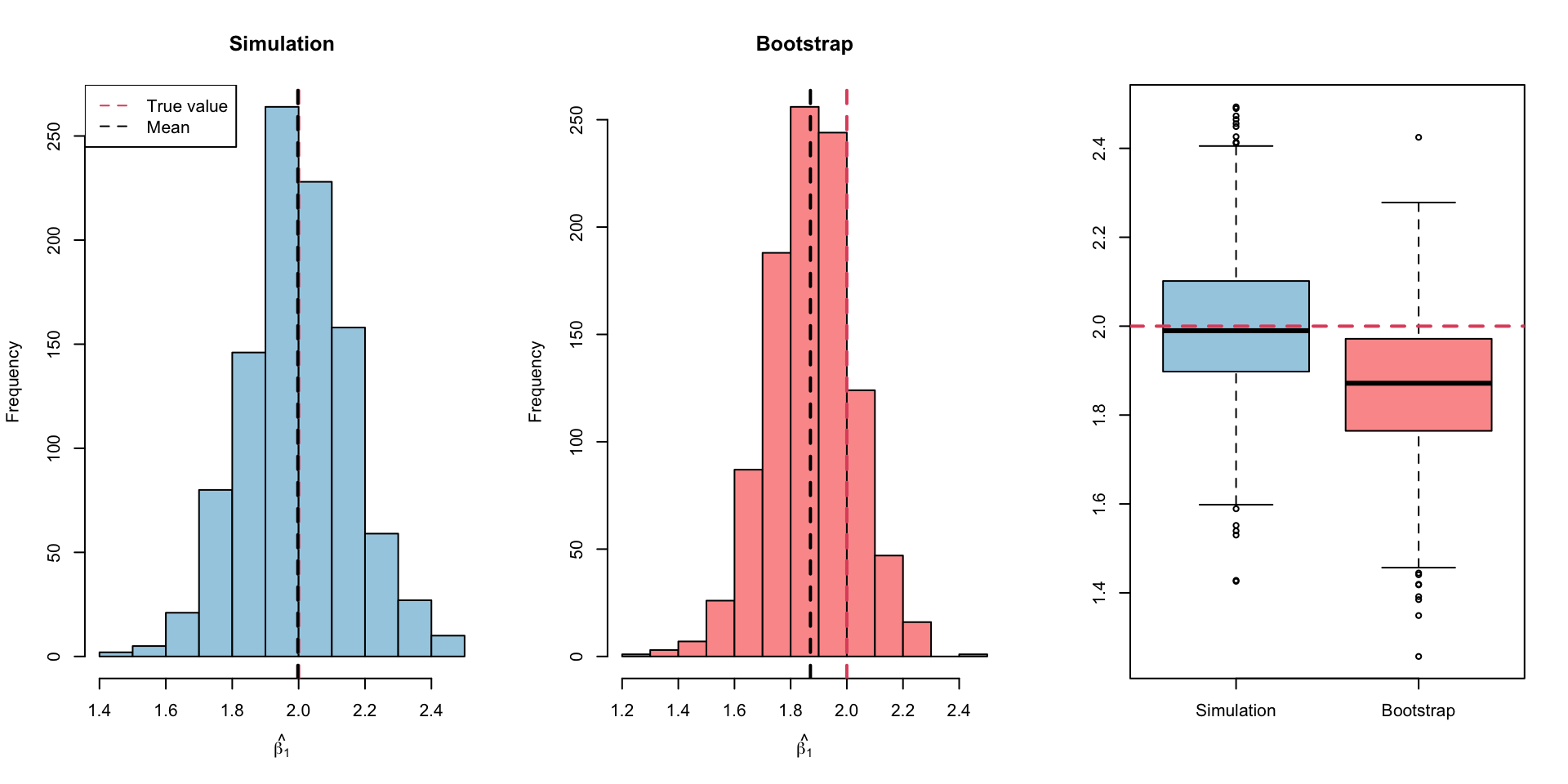
Simulated vs Bootstraped

Left: A histogram of the estimates of \(\mu\) obtained by 1000 simulated data sets from the true population (where \(\mu =0\)). Right: A histogram of the estimates of \(\mu\) obtained from 1000 bootstrap samples from a single data set of size 30.

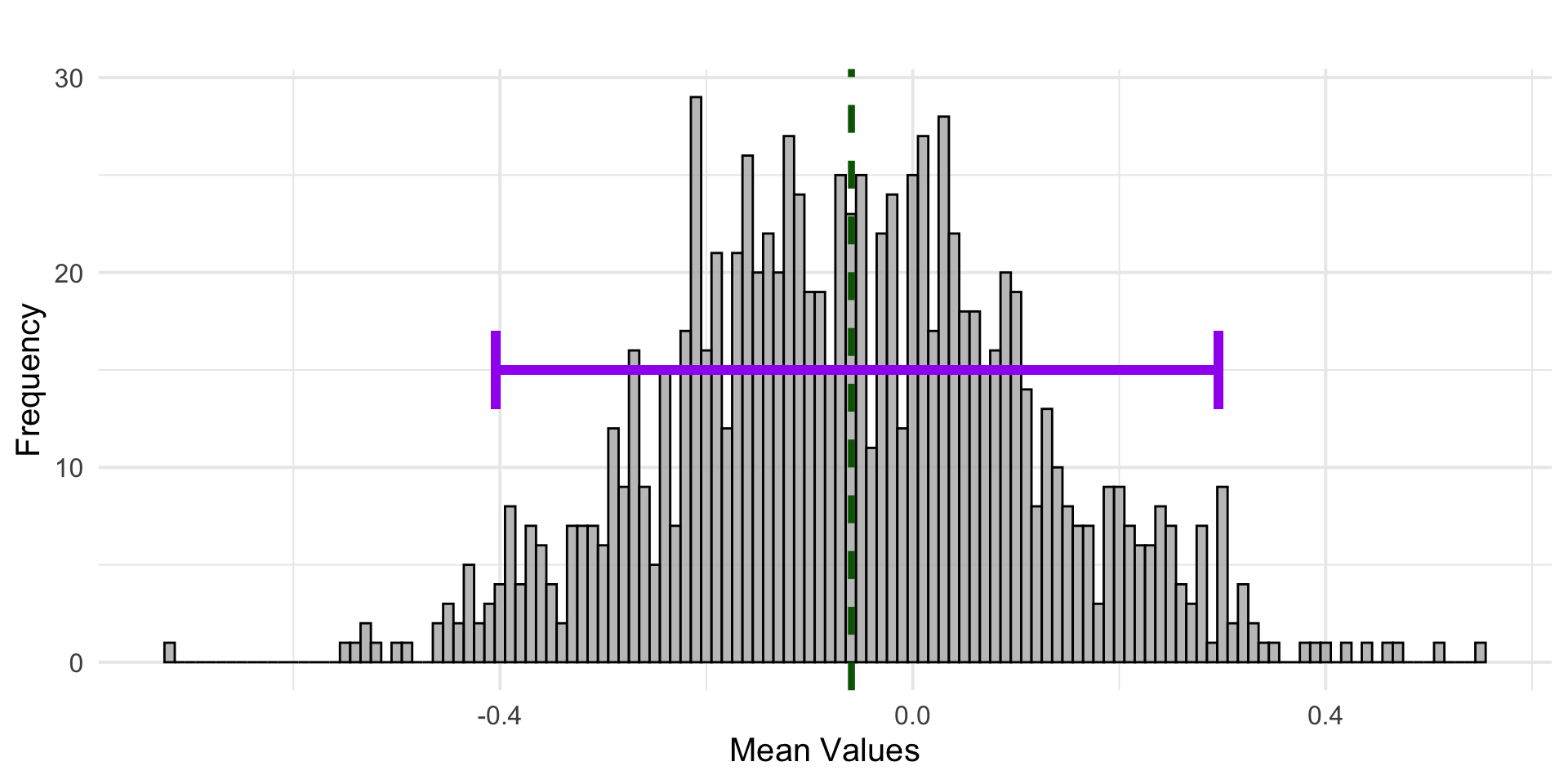
Bootstrap Confidence Interval

A histogram of the estimates of \(\bar{X}\) obtained by 1000 simulated data sets from the true population (where \(\mu =0\)). The purple indicates the 95% confidence interval as estimated from the bootstrap samples.

Why Bootstrap?

• The bootstrap used to estimate confidence intervals for parameters, especially when:

  • The distribution of the statistic is unknown or complicated.
  • The sample size is small, and parametric methods may not be reliable.

• More generally, it offers a flexible, non-parametric way to estimate uncertainty for statistical estimates, e.g. standard errors and bias of parameter estimates.

• In practice, resampling from the population is costly so we’re usually just stuck with a single sample.

• Furthermore the sampling distribution may not be known.

• No assumptions

Now we can get CI, p-values without the theoretical knowledge of the sampling distribution

• even if we know the sampling distribution (like in regression), sometimes it relies on CTL and we need a sufficiently large sample before it kicks in

• For emsemble methods, the bootstrap will be used to help avoiding overfitting and improves the stability of machine learning algorithms.

The name:

• “to pull oneself up by one’s bootstraps” from the fable from the 18th century. Meaning: to succeed or elevate yourself without any outside help.

• we’re going to the use the data we’ve got to get more information about our estimator

Bradley Efron at Stanford University in California won the 2018 International Prize in Statistics for pioneering the bootstrap method [Nature News Article]

What is Bootstrap?

Definition: Bootstrapping involves repeatedly sampling with replacement from a dataset to create multiple bootstrap samples.

Purpose: It estimates the distribution of a statistic (e.g., mean) by simulating many possible outcomes.

Key Concepts:

• Sampling with replacement vs. without replacement.
• How bootstrapping can be used in machine learning to estimate performance metrics.

Steps

Consider some estimator \(\hat \alpha\). For \(j = 1, 2, \dots B\) ¹

1. take a random sample of size \(n\) from your original data set with replacement². This is the \(j\)th bootstrap sample, \(Z^{*j}\)
2. calculate the estimated value of your parameter from your bootstrap sample, \(Z^{*j}\), call this value \(\hat \alpha^{*j}\).

Estimate the standard error and/or bias of the estimator, \(\hat \alpha\), using the equations given on the upcoming slides.

• Essentially we pretend that our data set is our population and we’re going to take repeated samples from that data set

1. \(B\) is usually quite is large (1000, 5000 are standard amounts)

2. where \(n\) is equal to the number of samples in your original data set

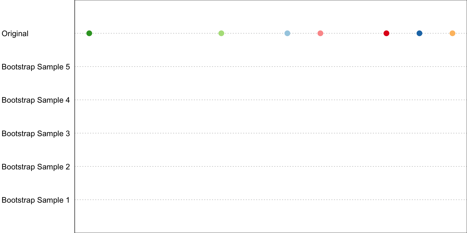
Sample with replacement

An illustration of sampling with replacement. The top row shows the original dataset, while the rows below represent different bootstrap samples. Each dot corresponds to a data point, with some points being selected multiple times (overlapping dots) and others not at all.

Some some samples might appear multiple times, and some not at all

Similar to cross-validation, bootstrapping involves resampling from a single dataset to simulate the presence of multiple datasets. However, unlike cross-validation, bootstrapping samples with replacement, meaning the same data point can be selected more than once in each resample.”

Bootstrap/full Estimates

Bootstrap Standard Error

Bootstrap estimates the standard error of estimator \(\hat \alpha\) using¹

\[\begin{equation} \hat{\text{SE}}(\hat \alpha) = \sqrt{\frac{\sum_{i=1}^{B} (\hat \alpha^{*i} - \overline{\hat \alpha})^2}{B -1}} \end{equation}\]

where \(\overline{\hat \alpha} = \sum_{j = 1}^B \hat \alpha^{*j}\) is the average estimated value over all \(B\) bootstrap samples.

\(\hat SE(\alpha)\) simply just sample sd for \(\alpha\)’s! (Recall the sample st. dev formula \(s = \sqrt{\frac{\sum (x_i - \overline x)^2}{n-2}}\))

1. AKA the sample standard deviation sd() of the \(\hat\alpha^{*i}\)s!

Bootstrap Bias

The bootstrap estimates the Bias of estimator \(\hat \alpha\) using:

\[\begin{align} \hat{\text{Bias}}(\hat \alpha) = \overline {\hat \alpha} - \hat \alpha_f \end{align}\]

where \(\overline{\hat \alpha} = \sum_{j = 1}^B \hat \alpha^{*j}\) and \(\hat \alpha_f\) is the estimate obtained on the original data set.

Usually i denote the estimator by capital letters (eg. \(\overline X\) and the observed value by lower-case (eg. \(\overline x\)). The this case \(\hat \alpha\) refers to the estimator and \(\hat \alpha_f\) refers to the estimate from the full (original) data.

Regression Example

We simulate 30 observations from a simple linear regression model with intercept \(\beta_0 = 0\) and slope \(\beta_1 = 2\). That is: \[Y = 2X + \epsilon\] where \(\epsilon \sim N(0, 0.25^2)\).

N.B. For ease of notation in the bootstrap section, I will denote \(\beta_1\) (and \(\hat \beta_1\)) by simply \(\beta\) (and \(\hat \beta\)).

As a simple example, the bootstrap can be used to estimate the standard errors of the coefficients from a linear regression fit.

In the specific case of linear regression, this is not particularly useful, since we saw in Chapter 3 that standard statistical software such as R outputs such standard errors automatically.

However, the power of the bootstrap lies in the fact that it can be easily applied to a wide range of statistical learning methods, including some for which a measure of vari- ability is otherwise difficult to obtain and is not automatically output by statistical software.

Data Generation

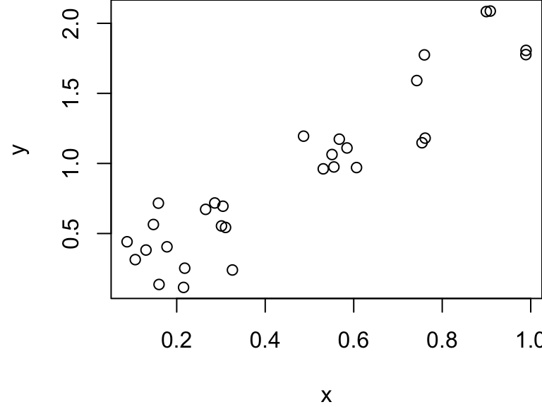
We generate a single sample from our population here:

set.seed(123978)
n = 30
beta1 = 2
sigma = 0.25 
x <- runif(n, 0, 1)
y <- beta1*x + rnorm(n, sd=sigma)
xy <- cbind(x,y)

Summary of Fit

And fit a simple linear regression model:

fullfit <- lm(y~x) 
(sfit <- summary(fullfit))

...

Coefficients:
            Estimate Std. Error t value Pr(>|t|)    
(Intercept)  0.05798    0.07773   0.746    0.462    
x            1.86641    0.14348  13.008 2.17e-13 ***
---
Signif. codes:  0 '***' 0.001 '**' 0.01 '*' 0.05 '.' 0.1 ' ' 1

Residual standard error: 0.2213 on 28 degrees of freedom
Multiple R-squared:  0.858, Adjusted R-squared:  0.8529 
F-statistic: 169.2 on 1 and 28 DF,  p-value: 2.172e-13
...

Sampling Distribution of \(\hat \beta_1\)

It can be shown that the sampling distribution of \(\hat \beta_1\) is given by a normal distribution centered at the true value, and standard error given below

\[\begin{align} \hat\beta_1 &\sim \text{Normal}\left(\beta_1, \dfrac{\sigma^2}{S_{xx}}\right) & \text{where } S_{xx} = \sum_{i=1}^n (x_i - \overline x)^2 \end{align}\]

Note that this is an unbiased with known standard error!

sampling distribution probability distribution of a given random-sample-based statistic.

Theoretical Bias and SE

In other words our we are using an unbiased estimator for slope (bias = 0) with the following theoretical standard error:

sxx <- sum((x - mean(x))^2)
(true.seb = sqrt(sigma^2/sxx))

[1] 0.162064

\[\begin{align} SE(\hat\beta_1)& = \sqrt{\dfrac{\sigma^2}{S_{xx}}} = \sqrt{\dfrac{0.25^2}{2.38}} = 0.1621 \end{align}\]

Estimates for a single fit

Notice that our summary output provides an estimate of the standard error of \(\hat \beta_1\) from the summary of the lm output (calculated using):

\[\hat{SE}(\hat\beta_1)=\sqrt{\frac{\sum_i\hat\epsilon_i^2}{(n-2)\sum_i(x_i-\bar x)^2}} = 0.1435\]

Since we’ll need this later, note the following estimate on the original data: \(\hat \beta_1 = 1.8664\) (we’ll call this \(\hat\beta_f\) later)

This is what you see in the table for SE(b1)

we have our true value for se = 0.1621 and our true value for bias = 0, now lets see how the bootstrap does at estimating

Bootstrap Simulation

• While it is a fairly routine to arrive at these equations, this might not be the case for more complicated scenarios.

• As an exercise, let’s pretend that we do not know what the standard error and bias of our estimator \(\hat \beta_1\) is.

• Instead, let’s estimate the bias (which we know should be 0 since \(\hat \beta_1\) is and unbiased estimator) and standard error using the bootstrap method.¹

1. Recall I will be dropping the subscript in \(\beta_1\) to make things more readable

R code

set.seed(311)
bootsamp <- list()
bootsmod <- list()
bootcoef <- NA
B = 1000 # number of bootstrap samples to be taken
for(i in 1:B){
  Zj <- xy[sample(1:n, n, replace=TRUE),]
  bootsamp[[i]] <- Zj # store our bootstrap samples in a list
  bootsmod[[i]] <- lm(Zj[,2]~Zj[,1])
  bootcoef[i] <- bootsmod[[i]]$coefficient[2] # ^betaj
}

Alternatively, you could use the boot() function from the boot package to do this.

The trick is going to be in creating a function (or apply the $ on some output) for obtaining that estimate

Bootstrap Estimate for Bias

We now have \(B = 1000\) estimates for \(\beta\) stored in bootcoef = \(\{\hat \beta^{*1},\hat \beta^{*2}, \dots, \hat \beta^{*1000}\}\) and the following values

\[\begin{gather} \overline{\hat \beta} = \sum_{j = 1}^{B = 1000} \hat \beta^{*j} = 1.8704 \quad \hat \beta_f = 1.86641 \\ \text{Bias}(\hat \beta) = \overline {\hat \beta} - \hat \beta_f = 1.8704 - 1.8664 = 0.004 \end{gather}\]

where \(\beta_f\) is obtained from the summary of fit on the full (i.e. original unbootstraped) data.

Bootstrap Estimate for SE

And the estimate for SE is given by this:

(seb = sqrt(sum((bootcoef - mean(bootcoef))^2)/(B-1)))

[1] 0.1543347

sd(bootcoef) # equivalent to the above

[1] 0.1543347

\[\begin{align} \hat{\text{SE}}(\hat \beta) &= \sqrt{\frac{\sum_{i=1}^{B} (\hat \beta^{*i} - \overline{\hat \beta})^2}{B -1}} = 0.1543 \end{align}\]

Bootstrap vs Theoretical SE(\(\hat\beta_1\))

The bootstrap estimate (=0.1543) is closer to the theoretical value (=0.1621) that the estimate obtained in the lm summary table from the (single) original data set (= 0.1435).

- 0.1621-0.1435= 0.0186 off with our single estimate
- 0.1621-0.1543 = 0.0078 with our bootstrap estimate

Important

This estimate was created with no knowledge of the theoretical sampling distribution!!

Had we not known the theoretical sampling distribution for \(\hat \beta_1\) the bootstrap enables us to construct confidence intervals, perform hypothesis test (calculate \(p\)-values!)

Bootstrap vs Simulation-based SE(\(\hat\beta_1\))

• For fun, let’s compare this estimate to the simulation-based method which allows us to resample from this population many many times, …

for(i in 1:1000){
  newx <- runif(30, 0, 1)                     # generate a new sample
  newy <- 2*newx + rnorm(30, sd=0.25)         # for each iteration
  sample.i <- cbind(newx, newy)
  modnew[[i]] <- lm(sample.i[,2]~sample.i[,1])
  coefs[i] <- modnew[[i]]$coefficients[2]     # save estimate for beta1
}

Results (Visual)

• the center of this bootstrap is centered at the estimate of beta_1 for the full model

• the standard erros of the boxes are the same though!

• the center is kind of off but we’re not using bootstrap to estimate the \(\beta_1\) were just using it for estimating the \(SE(\beta_1)\)

Results (Table)

SE estimates from the simulation and the bootstrap simulation are very similar to each other and the theoretical value (=0.162)

Estimate/ R Code	Description
0.143 = from output table summary(fullfit)	Estimate from a single fit on the full data
0.154 = sd(bootcoef)	Bootstrap estimate obtained from 1000 bootstrap samples
0.160 = sd(coefs)	Standard errors obtained from resampling from the population 1000 times.

Comments

• Note that the center of the bootstrap histogram is centered at \(\hat \beta_f\), the estimate obtained using the full data, rather than at \(\beta_1 = 2\) (the true simulated value).

• While we will use the bootstrap to estimate the SE of our estimator, typically the point estimate will be given by the estimate obtained using the full data, rather than say the mean of the bootstrap estimates.

bootstrapping is the predominant nonparametric method used for bias and standard error calculations.

iClicker

Resampling with CV vs Bootstrap

What is the primary difference between the resampling technique used in cross-validation (CV) and the bootstrap method?

1. In CV, samples are drawn with replacement, while in the bootstrap method, samples are drawn without replacement.
2. In CV, samples are drawn without replacement, while in the bootstrap method, samples are drawn with replacement.
3. CV divides the dataset into distinct subsets (folds), while the bootstrap resamples with replacement from the original dataset.
4. CV divides the dataset into distinct subsets (folds), while the bootstrap resamples without replacement from the original dataset.

iClicker

Goals of CV vs Bootstrap

What is the primary difference in the goals of CV and the bootstrap method?

1. CV aims to estimate the variability of a statistic, while the bootstrap is used to estimate the model’s predictive performance.
2. CV focuses on estimating model performance by minimizing overfitting, whereas the bootstrap is used to estimate the variability of a statistic or parameter.
3. Both CV and the bootstrap are used for estimating the model’s predictive performance.
4. CV and the bootstrap both aim to reduce the bias of an estimator.

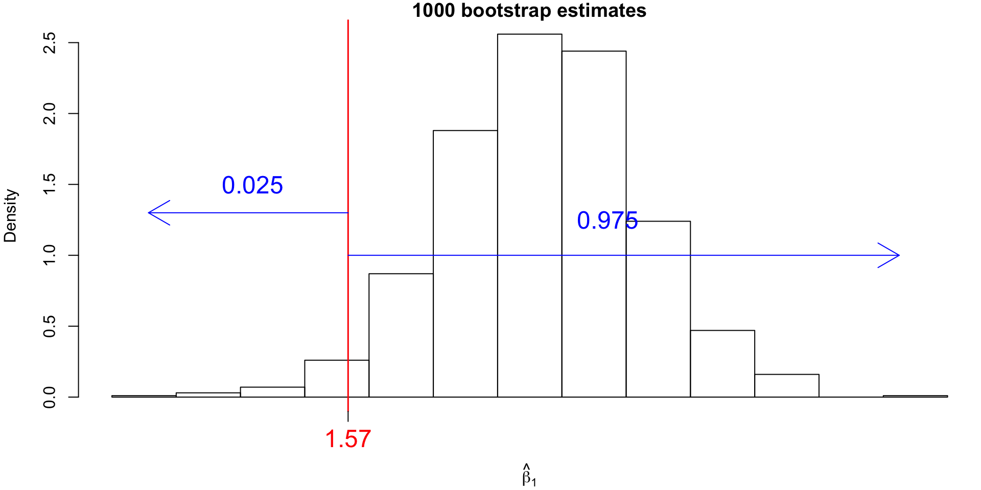
Computing Bootstrap CI

• We alluded to the potential of computing confidence intervals (CI) with the bootstrap.

• We already saw how the \(B\) bootstrap estimates of parameter \(\alpha\) provide an empirical estimate of the sampling distribution of estimator \(\hat \alpha\).

• To obtain confidence intervals from this empirical distribution, we would simply finding appropriate percentiles.

allows us to do inferential statistics

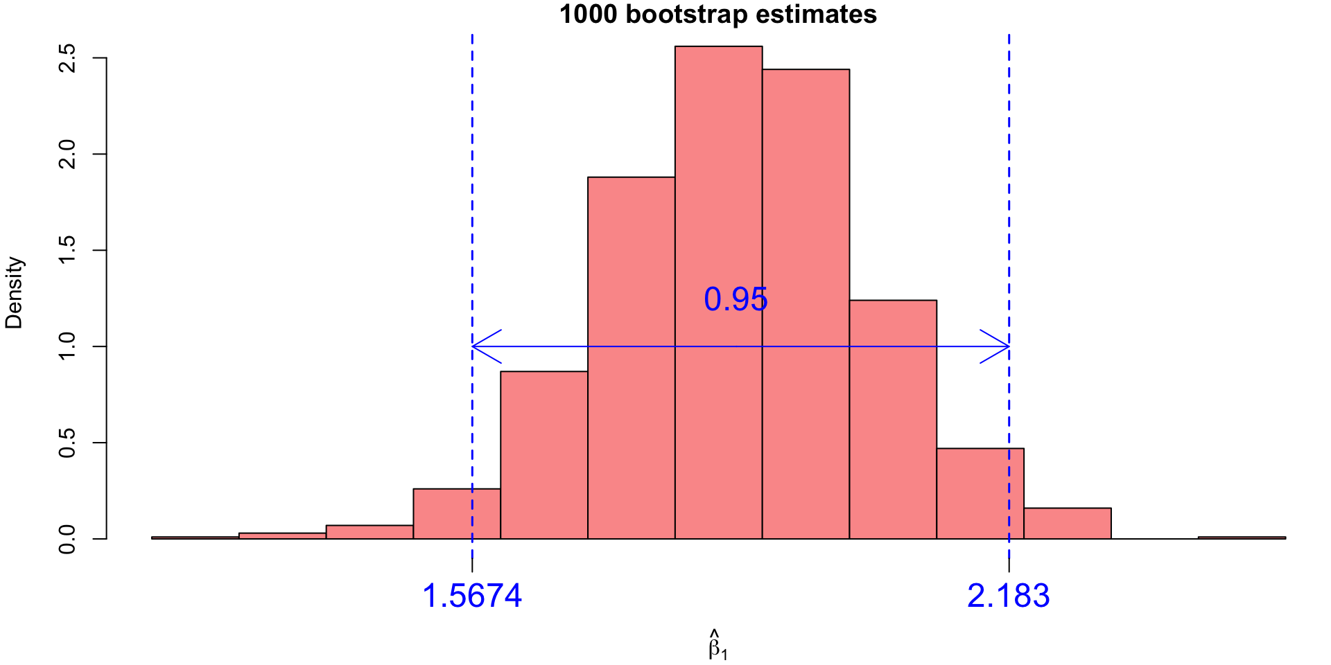
Bootstrap Confidence Intervals (CI)

For our example, the 95% bootstrap CI for \(\beta_1\) would correspond to the 25th value and the 975th value of the sorted bootstrap estimates.

quantile

These values can be found using the quantile() function:

quantile(bootcoef, .025) ; quantile(bootcoef, 1-.025) 

    2.5% 
1.567437 

   97.5% 
2.182977 

Estimated CI

So we have a 95% CI for true \(\beta_1\) lying within the interval: \[(1.5674, 2.183)\]

Quote

Statistical ‘rock star’ wins coveted international prize

The bootstrap is rarely the star of statistics, but it is the best supporting actor (Dr. Bradley Efron)

You can hear Dr. Brad Efron speak about the bootstrap here.

Dr. Efron gives a nice interview with the ILSR authors here.

• “inventer” of the bootstrap dr. bradley efron a statistician at Stanford
• wins the statistics version of the “nobel prize”: Internation Prize in statistics in 2018
• SE/CIs are ubigquitous in applied papers across natural science and for complex models with no closed-form soltuions, they’ll use the bootstraped SE/CIs

Ensemble Methods (e.g., Bagging)

• Bootstrap Aggregating (Bagging): One of the most common applications of bootstrapping is in bagging (Bootstrap Aggregating). In bagging, multiple bootstrap samples are drawn from the training data, and separate models are trained on each bootstrap sample. The predictions from these models are then averaged (for regression) or majority-voted (for classification) to create a more stable and accurate prediction.

  • Example: Random Forests is a popular bagging algorithm where decision trees are trained on different bootstrap samples, and predictions are averaged over all trees. This reduces variance and prevents overfitting.

  • Benefit: Bootstrapping helps ensure that each model in the ensemble is trained on slightly different data, which increases the diversity of the models and reduces the model’s variance.