Data 311: Machine Learning

Lecture 8: Cross Validation and Data Splitting

Dr. Irene Vrbik

University of British Columbia Okanagan

Introduction

• In this lecture we’ll be looking at a resampling method called cross validation (or CV for short)

• This technique will be used for validating/accessing our model by providing an estimate of model performance on unseen data (i.e. not used in training).

• By the end of this lecture, you should understand the difference between training, validation, and test datasets, the need for these splits, and how to implement CV.

• we have done this estimate before with a training/testing set, but as we will see, CV will have some benefits over this approach.
• Consequently, CV will be an indispensable tool for helping us choose between various modelling options.

Metrics for Model Assessment

For regression we aim to reduce the test MSE \[MSE = \frac{1}{m} \sum_{i=1}^m (y_i-\hat y_i)^2\]

For classification we may consider the test error rate \[\frac{1}{m} \sum_{i=1}^m I(y_i \neq \hat y_i)\]

Where \(1, \dots, m\) denotes unseen test observations that not used in the model-fitting process.

test error = misclassification rate of the error.

I use \(N\) to suggest that we want to minimize these for the population rather than just the sample we have on hand.

Recall

• Ideally, we could fit our model on a sample of data, and then compare the predictions from the estimated model on a very large data set (not used in fitting) to estimate the MSE¹.

• If we only have one sample, we often split it into a training set (used to fit the model) and testing set (used to estimate the test MSE).

• This train/test split approach is sometimes referred to validation approach.

we’ve used this approach before but i’ve never called it by this name: validation approach

1. We’ll start with MSE in the regression setting and see how these concepts can be extended to classification.

Training vs Test-set Performance

Recall: training error rate often is quite different from the test error rate [Image source]

• recall the diff between training and test error

• training error can dramatically underestimate test error.”

  • low = regression with a low number of predictors

  • high = large number of predictors

• for most models the training error will go down as complexity increases

• RIGHT: overfitting LEFT: underfitting

• Bias = how far off on average the model is from the truth
  Variance: how much the variance varies around its average

Validation Approach

Train/Test Split

set.seed(1234) # for reproducibility (eg. student number)
N = 200        # total number of obs. in our data set

# Randomly sample 80%/20% for training/testing
tr.ind <- sample(N, 0.8*N, replace=FALSE)
te.ind <- setdiff(1:N, tr.ind)

tr.ind

2, 3, 4, 6, 7, 8, 9, 10, 11, 14, …

te.ind

1, 5, 12, 13, 15, 18, 24, 31, …

In this case, we fit the model with samples with index tr.ind and estimate the MSE using samples with index te.ind

By now, we have experience splitting our data set randomly into non-overlapping training and testing sets:

Validation Approach Schematic

A schematic display of the validation set approach. A set of N observations are randomly split into training set (shown in red, containing \(n\) observations 2,3,4,6,7,8,9,10,11,14,…, among others) and a validation set (shown in blue, containing \(m\) observation 1, 5, 12, 13, 15, 18, 24, 31, 33, among others). The ML method is fit on the training set, and its performance is evaluated on the validation set.

this is a one-stage process

Can you think of any limitations/issues with this this method?

Any concerns? - Not a great option with small data sets - how do we decide on 80% (might need a minimum number to fit the model)

3. high variability it’s still just one sample, (if i do it again, i might get a completely different answer)
4. high bias (WASTEFUL) we’re throwing away or leaving out a lot of the data in the fitting process, and we know from intro stat that more data is generally better in terms of estimating a population parameter.
   

ISLR Train Test Figure

jump forward to cross-validation approach

ILSR Fig 5.2 Compares linear vs. higher-order polynomial terms in Linear Regression Left: Validation error estimates for a single split into training (196 obs.) and validation (196 obs.) sets. Right: The validation method was repeated ten times, each time using a different random split of the observations into a training set and a validation set. This illustrates the variability in the estimated test MSE from this approach applied to the Auto data set.

• Compares linear vs. higher-order polynomial terms in Linear Regression
• comparing with validation approach (no resampling) the MSE test is highly variable
• the “best” model changes from split to split
• this approach tends to overestimate the test error rate since much of the data is hidden in the fitting process (maybe half)

Validation approach

• The dataset is split into two subsets: a training set and a validation set.

• The model is trained on the training set and evaluated on the validation set to tune the model’s hyperparameters.

• There is no separate test set in this approach, which means you are using the validation set both for tuning and evaluation, which can lead to biased performance estimates.

Validation Approach: some problems

• High Variance: Results depend heavily on how the data is split.

• Inefficient Use of Data: Less data is available for training, especially with small datasets.

• Overfitting Risk: The model may overfit to the validation set.

• No Separate Test Set: Leads to biased performance estimates.

• Single Evaluation: One run may not reflect true generalization.

• Data leakage: the model “learns” from data it shouldn’t have access to during training which may lead to overly optimistic performance estimates

1. Since the model is evaluated on a single validation set, the performance estimate can vary significantly depending on how the data is split. Different random splits may yield different results, leading to unreliable estimates of model performance.

2. By splitting the data into just a training and validation set, you’re not using all available data for training. This is especially problematic with small datasets, where reducing the size of the training set can hurt model performance.

3. As the model is tuned using the validation set, there is a risk that the model may overfit to this specific data subset, making it less effective on truly unseen data.

4. The lack of a separate test set means the validation set is being used for both tuning and evaluation. This can lead to biased performance estimates, as the model may perform well on the validation set but poorly on new, unseen data.

5. You get only one point of evaluation for the model. This single validation score might not reflect the true performance, as it could be too high or too low purely by chance.

(Goodhart’s law) is an adage often stated as, “When a measure becomes a target, it ceases to be a good measure”.

Overall, these issues make the validation set approach less reliable compared to more robust methods like cross-validation or the train-validation-test split.

Multiple are needed to ensure that differences between models are not due to random variation in the test data.

Resampling Methods

Solution: training-validation-test split with multiple evaluations.

While we typically don’t have of multiple sets of data, we can fudge it using resampling methods which involves:

1. repeatedly drawing samples from a training set
2. refitting a model of interest on each sample

Bonus: this will provide additional information about the fitted model that we would not otherwise get.

Wikipedia Definition

1. The model is initially fit on a training data set
2. Successively, the fitted model is used to predict the responses for the observations in the validation data set.
3. Finally, the test data set¹ is used to provide an unbiased evaluation of a final model fit on the training data set.

⚠️ The ISLR textbook makes no distinction between the test set and validation set.

1. If the data in the test data set has never been used in training (for example in cross-validation), the test data set is also called a holdout data set.

Test/Validation/Test

All the data

0. Split the data into training, validation, and test sets (a common choice for this might be 70-10-20)

Training

valid.

test

1. Training Set: The portion of the dataset used to train the machine learning model. The model learns patterns and relationships from this data.

2. Validation Set: A separate subset used to tune the model’s hyperparameters and make decisions like model selection. It helps prevent overfitting but is not used for final evaluation.

3. Test Set: A completely independent subset used only after model training and tuning to assess the model’s performance on unseen data. It provides an unbiased estimate of how well the model generalizes.

Hide the Test set

Train, tune, and model-select with these:

Training

valid.

Used only after tuning/selection. Used to provide an unbiassed estimate of how well the model generalizes

test

Train, tune, and model-select with these:

Training

valid.

But this is still just one evaluation! We want to be able to do this multiple times. So we do something like this…

this solves the data leakage problem and lack of test set.

but we do not want to evaluate the candidate models once. so it doesn’t solve the variablity problem.

K-fold Cross-Validation

Training\(_1\)

valid.\(_1\)

Training\(_2\)

valid.\(_2\)

Train\(_2\)

Training\(_3\)

valid.\(_3\)

Training\(_3\)

Training\(_4\)

valid.\(_4\)

Training\(_4\)

Training\(_5\)

valid.\(_5\)

Training\(_5\)

Training\(_6\)

valid.\(_6\)

Training\(_6\)

Train\(_7\)

valid.\(_7\)

Training\(_7\)

valid.\(_8\)

Training\(_8\)

we do not want to evaluate the candidate models once. Instead, we prefer to evaluate each model multiple times with different dataset and take the average score for our decision.

So in this case, we’d have 8 different runs, and each data point will have a turn at belonging to the validation set.

The trick of \(k\)-fold (k = 8 here) to resample the same dataset multiple times and pretend they are different.

K Iterations (K-Folds): The dataset is divided into k equal-sized “folds” (in this example, k = 8). Each fold is used as a validation set once, while the remaining folds are combined to form the training set.

• 1st iteration: The first fold (in blue) is used as the validation set, while the remaining folds are used for training the model. The performance of the model on this validation fold is recorded as Performance₁.
• 2nd iteration: The second fold is used as the validation set, and the others for training. This gives Performance₂.
• The process repeats for all folds (3rd, 4th, … 8th), each time using a different fold as the validation set, while the rest are used for training.

Key Takeaways:

• Each fold gets a chance to be used as both training and validation data, which provides a better estimate of the model’s ability to generalize to unseen data.
• This method helps reduce bias from a single split and variance by considering multiple data splits.

Steps of K-fold CV

Step 0: Divide dataset into \(k\) equal-sized “folds”; each fold is used as a validation set once, while the remaining folds form the training set

1. 1st iteration: The first fold (in blue) is used as validation set\(_1\), while the remaining folds are used for training the model. The performance of the model on this validation fold is recorded as Performance₁.

2. 2nd iteration: The second fold is used as validation set\(_2\), and the others for training. This gives Performance₂.

The process repeats for all \(k\) folds, each time using a different fold as the validation set, while the rest are used for training.

The image on the previous slide shows the process of \(k\)-fold cross-validation.

CV Performance

After completing all \(k\) iterations, the performances from each fold are averaged to get a more reliable estimate of the model’s performance across different subsets of the data. Source of image: [Zitao’s Web]

this cv estimate of error will be more reliable than the test set one we were doing earlier which just relied on one random split - plus it means we don’t have to peak at the test set yet!

Retrain

Once we select a model from cross validation, we may want to retrain the model on the complete non-test samples (since combining the training and validation dataset can produce a better model since we have more data)

Training

valid.

test

Re-training selected model

test

Final model testing

• Once we have refitted the selected model on the non-test examples, we use the test dataset for unbiased final evaluation (e.g. \(MSE_{test}\) or test error)

• The test dataset, untouched until now, estimates model performance on unseen data and checks for overfitting¹.

The test dataset used for evaluation is independent from the validation sets we used in cross validation.

they are different because we do not want data leakage

Overfitting happens when a model performs exceptionally well on the training data but fails to generalize to new, unseen data. When we evaluate the model on the test dataset, it reveals whether the model has learned the underlying patterns or if it has simply memorized the training data.

1. If the performance on the test set is much worse than on the training/validation sets, it indicates that the model may be overfitting.

Summary of steps

1. Training Phase: Use Resampling Methods to obtain multiple training sets to train candidate models.
2. Model Evaluation: Instead of evaluating candidates once, evaluate each model multiple times with different validation sets.
3. Model Selection: Choose the best performing model based on the average validation scores.
4. Retrain: Combine training and validation sets (non-test set) for final training.
5. Final Model Testing: Evaluate the model’s performance on the test dataset

Average the scores to make a better decision.

Resampling Methods

• \(k\)-fold cross-validation (CV) is one of the most commonly used resampling methods

• Resampling methods involve repeatedly drawing samples from a dataset and training the model on different subsets of data to evaluate its performance.

• Another popular choose is Leave-one-out CV

• Next lecture we’ll discuss another resampling method called the bootstrap

The model is trained and validated on different “resampled” subsets of the data in each iteration, without the need to collect new data.

Today we focus on CV which can be used:

• to assess model performance (eg. estimate test MSE),
• perform model selection (eg. choose \(k\) for knn)
• model comparison (choosing between method 1 and 2)
• provide standard deviation and bias of our parameter estimates

• expensive because they involve fitting the same statistical method multiple times using different subsets of the training data.
• cv can be used to estimate the test error to eval performance
• The bootstrap is used in several contexts, most commonly to provide a measure of accuracy of a parameter estimate/learning method (estimate variance of estimators)

Leave One Out Cross-Validation

Leave One Out Cross-Validation (LOOCV) is a special case of \(k\)-fold CV; namely, where \(k\) equals the number of data points in the dataset.

1. The dataset is split into \(n\) folds, where \(n\) is the number of data points.

2. In each iteration, 1 data point is used as the validation set, and the remaining \(n-1\) data points are used as the training set.

• Unlike the validation approach, LOOCV systematically creates multiple training sets¹ of size \(n - 1\) each having a validation (i.e. testing) set with a single observation \((x_i, y_i)\)

• Unlike the validation approach the subsets will not be a comparable size but rather a single observation \((x_i, y_i)\) for the validation set, and the remaining observations making up the training set.

• hence we we are “holding out” one observation.

1. this method will split our data into training and validation set \(n\) times (where \(n\) is our sample size).

LOOCV approach

Full sample index (1, 2, … , 200) is systematically divided into:

	Index
CV Set	Training	Validation*
1	2, 3, 4, ..., 200	1
2	1, 3, 4, ..., 200	2
3	1, 2, 4, ..., 200	3
...	...	...
200	1, 2, 3, ..., 199	200

Rather than test set we may use “validation” or “hold-out” set

LOOCV Schematic

A schematic display of LOOCV. A set of n data points is repeatedly split into a training set (shown in red) containing all but one observation, and a validation set that contains only that observation (shown in blue). The test error is then estimated by averaging the n resulting MSE’s. The first training set contains all but observation 1, the second training set contains all but observation 2, and so forth.

• Notice how each CV set (i.e. each row) defines a non-overlapping partition of the data.

• IOW each observation is represented either in the training or validation set.

LOOCV Steps

Steps:

Create \(n\) training/validation sets, then for each set:

• Fit the model to the training set

• Use the fitted model from 2. to predict the responses for the observation in the validation set.

• Record the validation set error.

The final performance is the average of the performance scores from each iteration.

CV Estimation

• If our response is quantitative, our validation set error can be assessed using the MSE.

• For LOOCV the MSE corresponds to a single left out observation \(x_i\) will be defined as \(MSE_i = (y_i-\hat y_i)^2\) where \(\hat y_i\) is the prediction found from the \(i^{th}\) fitted model.

• We can then estimate the MSE of the model using \[CV_{(n)} = \frac{1}{n} \sum_{i=1}^n MSE_i\]

\((n)\) in the subscript denotes how many CV/validation sets we have

LOOCV Steps Visualized

Training Set	Prediction	Metric \(MSE_i\)
2,3,4, …, 199, 200	\(\hat y_1 = \hat f_{1}(x_1)\)	\((y_1 - \hat y_1)^2\)
1,3,4, …, 199, 200	\(\hat y_2 = \hat f_{2}(x_2)\)	\((y_2 - \hat y_2)^2\)
1,2,4, …, 199, 200	\(\hat y_3 = \hat f_{3}(x_3)\)	\((y_3 - \hat y_3)^2\)
\(\vdots\)	\(\vdots\)	\(\vdots\)
1,2,3, …, 198, 199	\(\hat y_{200} = \hat f_{200}(x_{200})\)	\((y_{200} -\hat y_{200})^2\)

Pros to LOOCV

1. Less bias: LOOCV uses almost all of the data to fit the model whereas the validation approach may only use 50% (which tends to lead to an overestimate of the test error).

2. Deterministic estimates: LOOCV always gives the same estimate because the partitions are not chosen randomly.

3. Very general: LOOCV¹ can be used with any kind of predictive modeling; logistic regression, LDA, you name it!

1. LOOCV tends not to overestimate the test error rate as much as the validation approach
2. validation approach will give you a different answer every time due to the randomness in the train/testing split
3. some methods will even have LOOCV built in

1. While the validation approach can be general as well, LOOCV has the added benefit of having more data which may be important for methods like QDA

Cons to LOOCV

1. Computationally demanding¹: LOOCV requires the model to be fitted \(n\) times which can be very costly if \(n\) is large and/or the model is slow to fit.

2. More variance since LOOCV estimates are highly correlated² \[\begin{align} \text{Var}(X + Y) = \text{Var}(X) + \text{Var}(Y) + 2\cdot\text{Cov}(X,Y) \end{align}\]

• Con 1: This can be very time consuming if n is large, and if each individual model is slow to fit (a shortcut exists for regression)
  • (consider \(n\)=1000 images!) or a model that takes 5 days to run a single model
  • wine data example took 30 seconds (which might not seem like a lot but its not that big of a data set)
  • there are some shortcuts for regression (see textbook)
• Con 2: But even though MSE1 is unbiased for the test error, it is a poor estimate because it is highly variable, since it is based upon a single observation
• usually k-fold with 5 or 10 is best

1. With least-squares linear or polynomial regression there is a mathematical shortcut that does not require us to refit the model

2. since they trained on an almost identical set of observations

Comments on k-Fold CV

• As mentioned earlier, \(k\)-fold CV is more general than LOOCV (with the added benefit of less variance)

• While \(k\) can be anything from 1 to \(n\), typically we use 5- or 10-fold CV.

• While we try to subdivide the data into equally-sized non-overlapping sets, sometimes that is impossible so we approximate¹

• Each set (or “fold”) takes a turn as the validation set, with the remainder of the data used to train the model.

• We usually shuffle the data before making the folds

• divide data into k groups, or “folds”
• typically k = 5 or 10

1. your sample size may not divide perfectly. For example if \(n=20\) and \(k=3\) (20/3 = 6.67) you might use two validation sets with 7 observations and one with 6

5-fold Visualization

A schematic display of 5-fold CV. A set of n = 20 observations is randomly split into five non-overlapping groups (or folds). Each of these folds takes a turn a validation set (shown in blue), and the remainder as a training set (shown in red). The test error is estimated by averaging the five resulting MSE estimates.

• Observations appear in exactly 1 validation set -LOOCV is a special case of k-fold CV in which k is set to equal n
• typically use k = 5 or k = 10.
• PRO there is much less overlap in these training sets than in LOOCV
• LOOCV is a special case of k-fold (when k = n)

Dataset Splitting: The original dataset is divided into k roughly equal-sized subsets or “folds.” Each fold contains a portion of the data, and typically, these subsets do not overlap.

Iterative Process: The cross-validation process is then performed iteratively for k rounds. In each round, one of the k folds is used as the validation set, and the remaining k-1 folds are used as the training set.

Model Training and Testing: The model is trained on the training set, and its performance is evaluated on the validation set. This performance metric (e.g., accuracy, mean squared error) is recorded for each round.

Average Performance: After all k rounds are completed, the performance metrics from each round are usually averaged to provide a single estimate of the model’s performance.

\(k\)-Fold split

Full Sample Index: 1, 2, … , 20, with \(k = 5\)

Training Set	Validation*
1, 2, 4, 5, 6, 8, 9, 11, 13, 14, 15, 16, 17, 18, 19, 20	3, 7, 10, 12
1, 3, 5, 6, 7, 8, 9, 10, 11, 12, 13, 15, 16, 17, 18, 20	2, 4, 14, 19
1, 2, 3, 4, 6, 7, 8, 9, 10, 11, 12, 14, 15, 17, 19, 20	5, 13, 16, 18
1, 2, 3, 4, 5, 7, 10, 11, 12, 13, 14, 16, 17, 18, 19, 20	6, 8, 9, 15
2, 3, 4, 5, 6, 7, 8, 9, 10, 12, 13, 14, 15, 16, 18, 19	1, 11, 17, 20

• Here the data set split evenly but remember there may be validation sets of slightly different size
• Note there different sizes will be taken into account in the weights of the CV estimates

5-fold CV Calculations

Where \(\hat f_j\) is the model fitted using all observations not in validation set (i.e. \(i \notin V_j\)).

Validation Set \(V\)	Prediction	Metric \(MSE_j\)
\(V_1\) = 3, 7, 10, 12	\(\hat f_1 (x_3, x_7, x_{10}, x_{12})\)	\(\frac{1}{4}\sum_{i\in V_1} (y_i - \hat y_i)^2\)
\(V_2\) = 2, 4, 14, 19	\(\hat f_2 (x_2, x_4, x_{14}, x_{19})\)	\(\frac{1}{4}\sum_{i\in V_2} (y_i - \hat y_i)^2\)
\(V_3\) =5, 13, 16, 18	\(\hat f_3 (x_5, x_{13}, x_{16}, x_{18})\)	\(\frac{1}{4}\sum_{i\in V_3} (y_i - \hat y_i)^2\)
\(V_4\) =6, 8, 9, 15	\(\hat f_4 (x_6, x_8, x_{9}, x_{15})\)	\(\frac{1}{4}\sum_{i\in V_4} (y_i - \hat y_i)^2\)
\(V_5\) =1, 11, 17, 20	\(\hat f_5 (x_1, x_{11}, x_{17}, x_{20})\)	\(\frac{1}{4}\sum_{i\in V_5} (y_i - \hat y_i)^2\)

\[\begin{align} \text{CV}_{(5)} = \frac{1}{5} \sum_{j=1}^5 MSE_j \end{align}\]

CV is the weighted average of the \(MSE_k\)

\(k\)-Fold Estimation

More generally, we can calculate the MSE for each validation set \(j\), for \(j = 1, \dots, k\) \[MSE_j = \frac{1}{n_j} \sum_{i \in j}(y_i-\hat y_i)^2\] where \(n_j\) is the number of observations in the \(j\)th validation set. A cross-validated estimate the MSE given by \[ CV_{(k)} = \frac{1}{k}\sum_{j=1}^k MSE_j \]

• This process results in k estimates of the test error, MSE1, MSE2, . . . , MSEk
• if k = 5, we run the model 5 times and obtain 5 mse est then average them
• denom is just saying number of obs in that validation set j (which may or may not be the same for each validation set if we have a data set that doesn’t divide perfectly)

ISLR Cross Validation Figure

jump back to validation approach

ILSR Fig 5.4 Cross-validation was used on the Auto data set in order to estimate the test error that results from predicting mpg using polynomial functions of horsepower. Left: The LOOCV error curve. Right: 10-fold CV was run nine separate times, each with a different random split of the data into ten parts. The figure shows the nine slightly different CV error curves. These are much less variable than the Validation Approach

• one curve of LOOCV since its deterministic
• 10-fold is stochastic so let’s run in a few times (nine times)
• While there is some variability in the resulting estimates for error they are much more stable than the validation approach
• The curve is telling us that a quadradic, cubic, quatric, quintic, sextic, septic, octic, nonic, decic (tenth-order) polynomial all preform similarly well on data it hasn’t seen.
• In the spirit of K.I.S.S and parsimony, this would give us some reason to choose a quadradtic (second-degree polynomial). Notably a 1st degree polynomal (linear regression) would not suffice

\(k\)-fold vs. LOOCV

Pros of \(k\)-fold

1. Less variance than LOOCV
2. More computationally feasible than LOOCV (\(k\) vs. \(n\) model fits)
3. Often gives more accurate estimates of test error than LOOCV.

Cons of \(k\)-fold

1. more bias than LOOCV when estimating MSE
2. Non deterministic estimate of the MSE (randomly spliting the data into \(k\) folds)

Pros 1. Since the mean of many highly correlated quantities has higher variance than does the mean of many quantities that are not as highly correlated, the test error estimate resulting from LOOCV tends to have higher variance than does the test error estimate resulting from k-fold CV. 3. this has to do with bias-var tradeoff

3. why (next slide?) Bias-Variance Tradeoff: LOOCV has lower bias but higher variance, whereas k-fold CV strikes a better balance between bias and variance.

Cons 1. k-fold is trained using less data so more bias towards overestimating the true MSE gives more accurate estimates of the test error rate than does LOOCV. - validation (high bias) sweet spot LOOCV (~unbiased)

Bias-Variance trade-off

LOOCV will have lower bias than does \(k\)-fold CV with \(k < n\), but LOOCV has higher variance.

Again we are seeing the bias-variance trade-off that we have discussed previously throughout the course!

- LOOCV less bias: uses almost all the data we have on hand
- LOOCV high variance: since the estimates are highly correlated (because the differ by a single observation)

Bias-Variance Tradeoff: LOOCV has lower bias but higher variance, whereas k-fold CV strikes a better balance between bias and variance.

(general recommendation on next slide)

k-fold or LOOCV?

• k-fold or LOOCV

k-fold or LOOCV?

• k-fold or LOOCV? ¹ What value of \(k\) is best?

• The ISLR authors argue that for intermediate values of \(k\), say 5 or 10, \(k\)-fold CV provides a better estimate of test error rate than LOOCV²

• In other words, the decrease in variance tends to outweigh the increase in bias when we chose 5/10-fold validation over LOOCV.

• generally speaking k-fold with 5 or 10 will tend to produced more accurate estimates of MSE than LOOCV.
  
• (Error = Var(g) + Bias(g)²) if we choose k-fold over LOOCV we increase Bias but decrease Var but the net loss will be bigger (generally speaking) when we choose k = 5, 10
• choice often between deterministic vs. non-deterministic method
• ILSR: shown empirically that 5/10fold CV suffer neither from excessively high bias nor from very high variance

1. LOOCV is a special case of k-fold CV

2. this point is debatable; see a discussion here

CV and Classification (LOO)

• CV (either \(k\)-fold or LOO) can be applied easily in a classification context as well.

• For instance, in LOOCV we can calculate cross-validated misclassification rates by replacing \(MSE_i\) with the validation misclassification rate (aka error rate \(\text{Err}_i\)) : \[ CV_{(n)} = \frac{1}{n} \sum_i^n \text{Err}_i = \frac{1}{n} \sum_i^n I(y_i \neq \hat y_i) \] where \(I(y_i \neq \hat y_i)\) is 1 if the left-out observation was misclassified using the \(i\)th model, and 0 otherwise.

CV and Classification (k-fold)

We divide the data into \(k\) roughly equal-sized parts \(C_1, C_2, \ldots, C_k\) where \(n_j\) is the number of observations in part \(j\): if \(n\) is a multiple of \(k\), then \(n_j = n/k\).

\[\begin{align} MC_j &= \frac{1}{n_j} \sum_{i \in j} I(y_i \neq \hat y_i) \\ CV_{(k)} &= \sum_{j=1}^k \frac{n_j}{n} MC_j \end{align}\]

• denom \(\sum_{i=1}^n I(i \in j)}\) is simply counting the number of observations in our validation set.
• numerator \(\sum_{i \in j} I(y_i \neq \hat y_i)\) is counting how many observations in our validation set were misclassified

We could also extend these CV estimates to other values such as log-loss

Model Selection

• We have just seen how we could use these methods to to assess model performance.

• Now let’s switch gears and see how these methods can be used for model selection.

• Now we can use cross-validation (CV) to compare and select the best-performing model among several candidates.

• In this case, we use CV to choose which value of k¹ for KNN performs the best in terms of generalization.

• model assessment we care what the MSE estimate was
• model selection we care where the minimum MSE estimate is
• These are the first systematic approaches we have for selecting among possible models!
• don’t be confused with the multiple use of \(k\)!

1. This k refers to the number of neighbours and has nothing to do with \(k\)-fold. I will try to distinguish these by using typewriter text when using k in reference to KNN.

iClicker

iClicker:

What is the primary purpose of the training dataset in machine learning?

1. To tune the model’s hyperparameters
2. To evaluate the final performance of the model
3. To train the model on a given dataset
4. To prevent overfitting during training

3. To train the model on a given dataset

iClicker

iClicker:

What is the key difference between a validation set and a test set?

1. The validation set is used for final model evaluation

2. The test set is used for hyperparameter tuning

3. The validation set is used for hyperparameter tuning, while the test set is for evaluating generalization

4. The validation set is larger than the test set

3. The validation set is used for hyperparameter tuning, while the test set is for evaluating generalization

iClicker

iClicker:

Which of the following best describes the concept of data leakage

A. Including irrelevant features in the training set B. Sharing test data with the training data C. Training on a small portion of data D. Using a non-random dataset split

2. Sharing test data with the training data

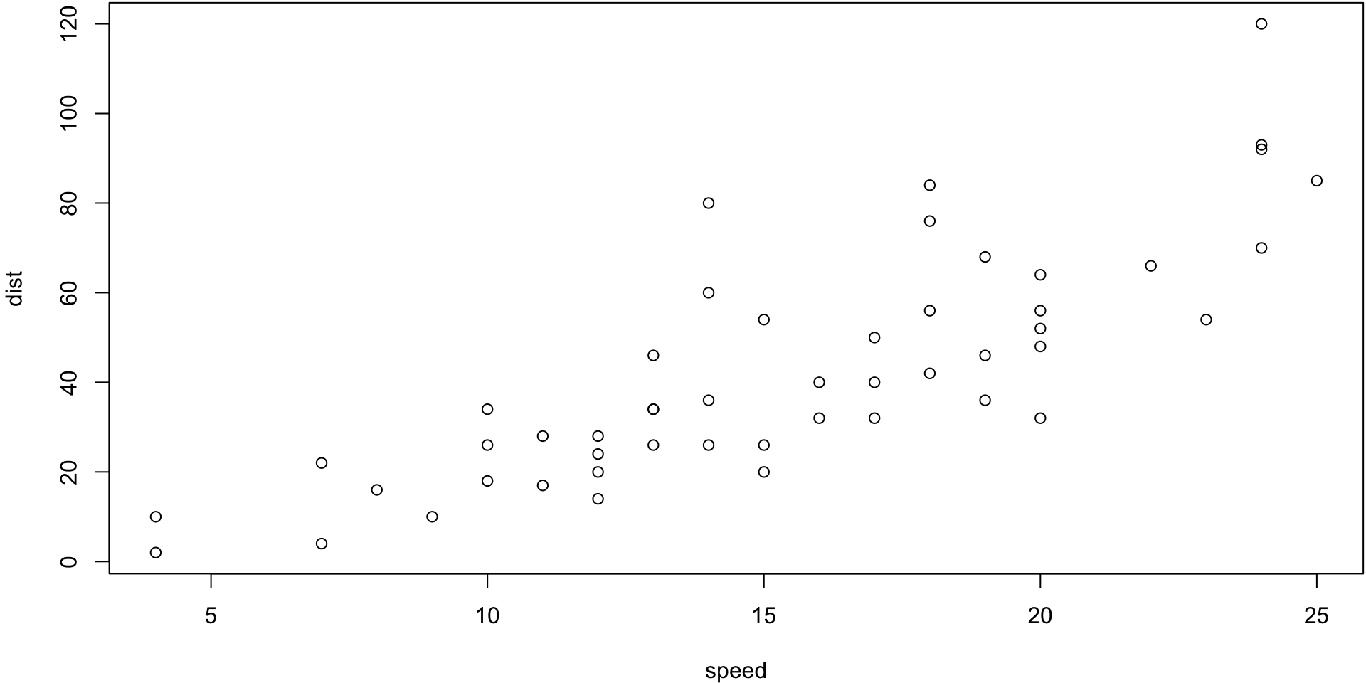
Cars Example

The cars data give the speed of 1920s cars (speed) and the distances taken to stop (dist).

KNN (from FNN package)

library(FNN)
knn.reg(train, test = NULL, y, k)

• train matrix or data frame of training set cases.
• test matrix or data frame of test set cases. A vector will be interpreted as a row vector for a single case. If not supplied, LOOCV will be done.
• y reponse of each observation in the training set.
• k number of neighbours considered.

Value returned: - PRESS the sums of squares of the predicted residuals = \(\sum_i^n (y_i - \hat y_i)^2\) (i.e the numerator of \(CV_{(n)}\))

Cross-validated estimates

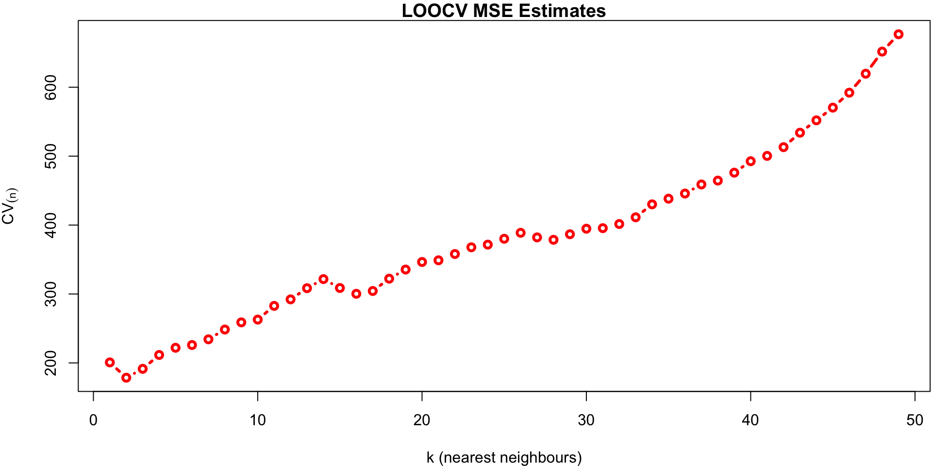
• We fit all possible k values (1 to 49 - the number of samples)

• If we don’t supply a test test, knn.reg performs LOOCV

• We plot the cross-validated estimates of MSE across all values of k each calculated using: \[CV_{(n)} = \frac{1}{n} \sum_{i=1}^n MSE_i\]

• where k is being used in the context of KNN.
• so there will be 49 different CV estimates (one for each value of k NN) Value returned: - PRESS the sums of squares of the predicted residuals = \(\sum_i^n (y_i - \hat y_i)^2\) (i.e the numerator of \(CV_{(n)}\))

k vs MSE plot

library(FNN)
data(cars, package="datasets")
attach(cars)
kr <- list()
predmse <- NA
for(i in 1:49){
  # LOOCV (default if no test set is supplied)
  kr[[i]] <- knn.reg(speed, test=NULL, dist, k=i)
  predmse[i] <- kr[[i]]$PRESS/nrow(cars) # LOOCV estimate for k = i
}
par(mar = c(4, 4.2, 1.1, 0.1))
plot(predmse, type="b", lwd=3, col="red", 
     ylab = expression(CV[(n)]), 
     xlab = "k (nearest neighbours)",
     main ="LOOCV MSE Estimates")

• this is estimating that true MSE curve (see fig 5.6 in ISLR)
• We want the model that minimizes the predicted MSE
• min is at \(k\)= 2

PRESS: the sums of squares of the predicted residuals. NULL if test is supplied.

k vs MSE plot

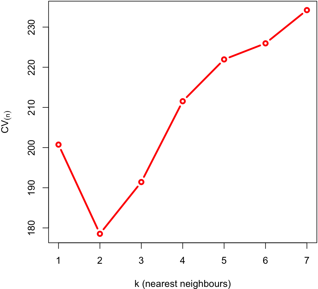
Zoomed in

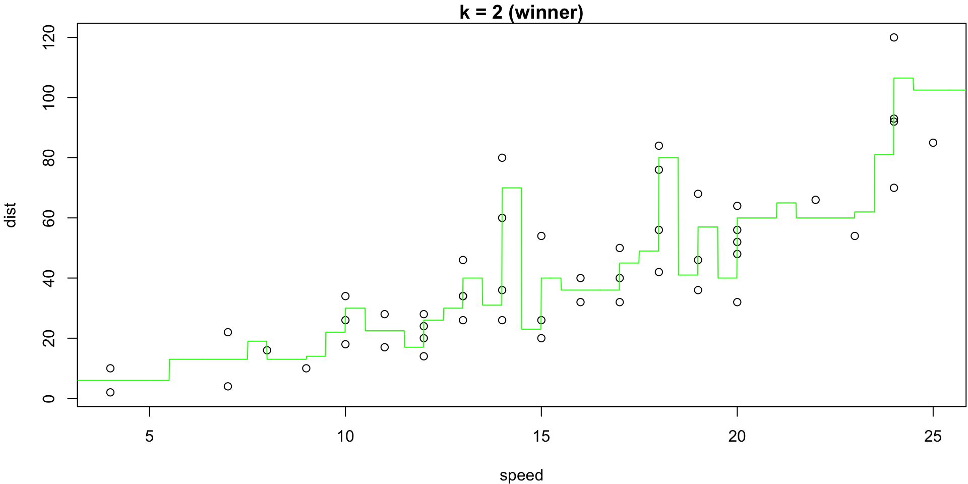
The minimum of that plot suggests that the best value of k is at 2.

Jump to compare with Regression MSE estimate.

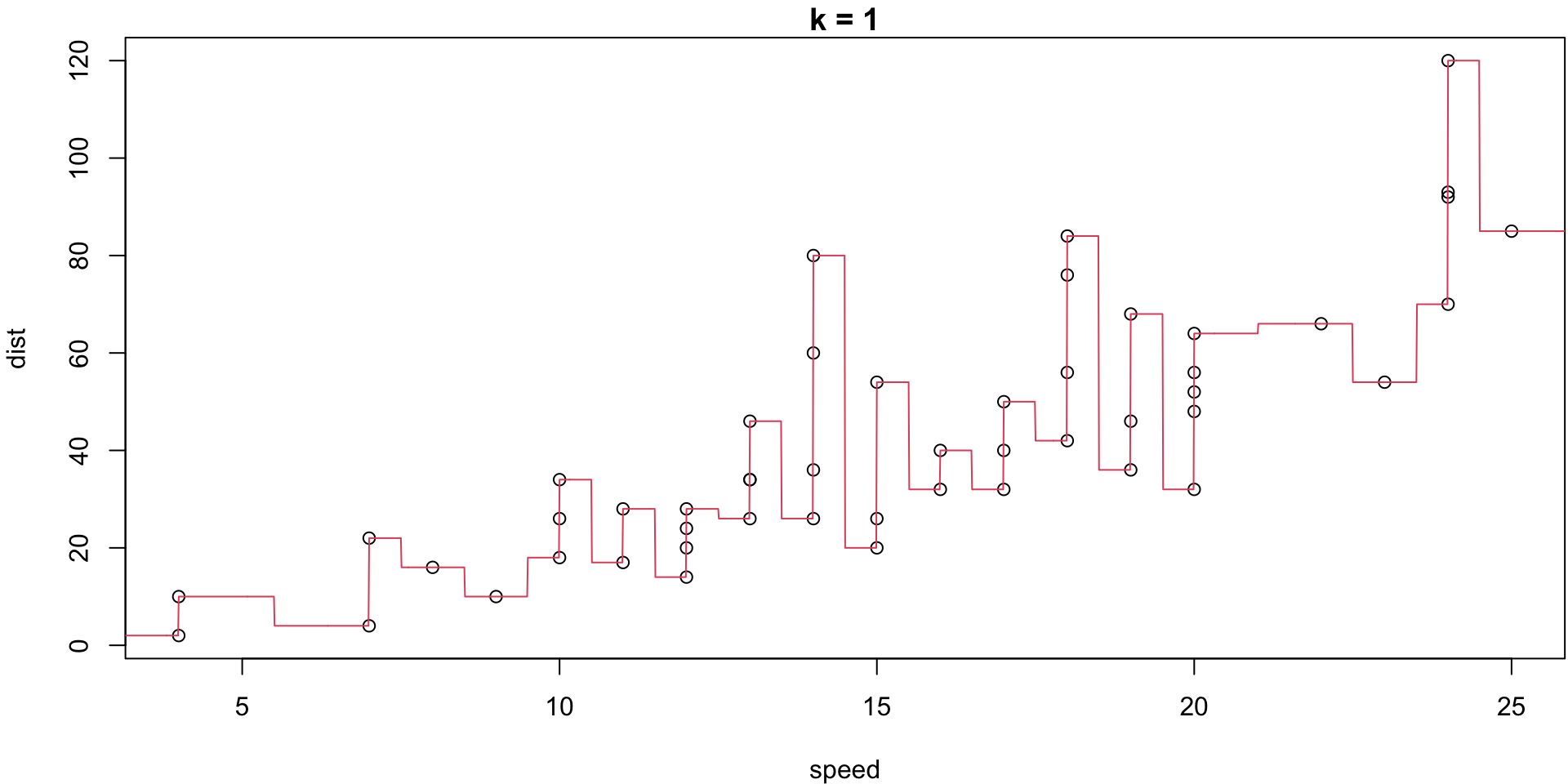
k = 1

Too flexible

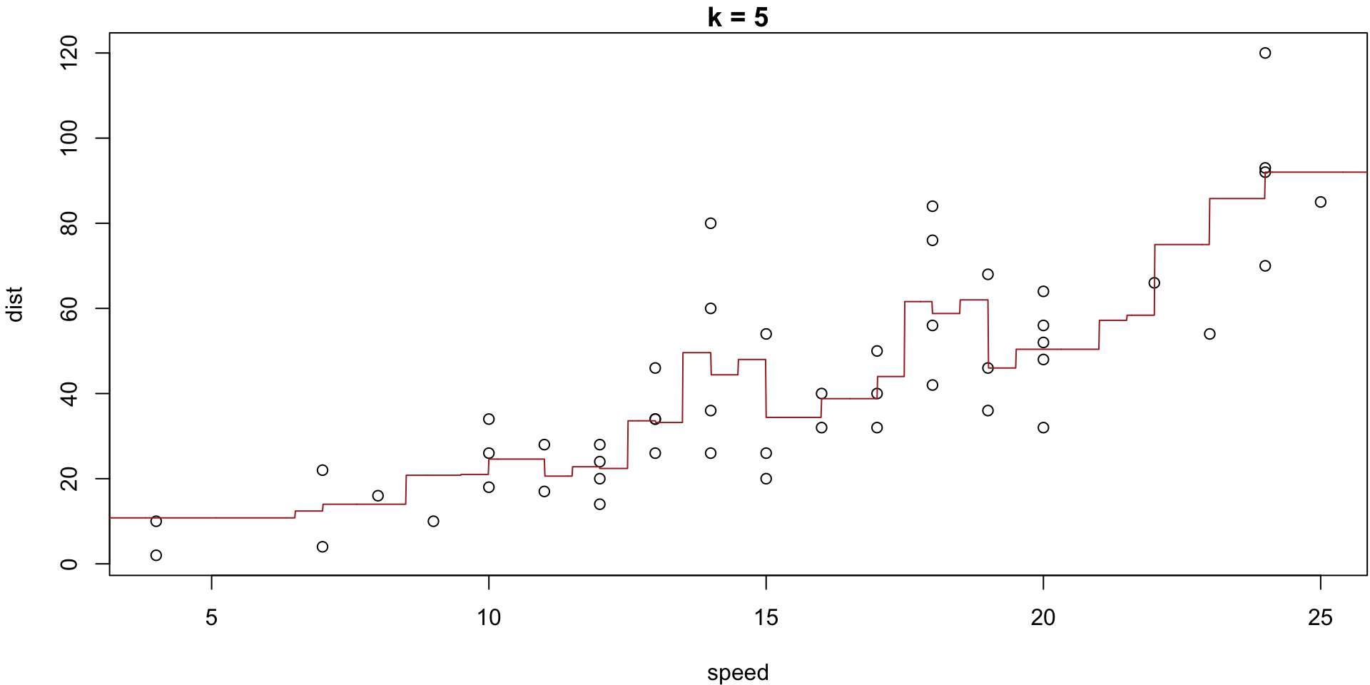
k = 5

• odd artifact of the data
• x’s (speed are discrete-ish)
• best model is to just take the average at each of these discrete values

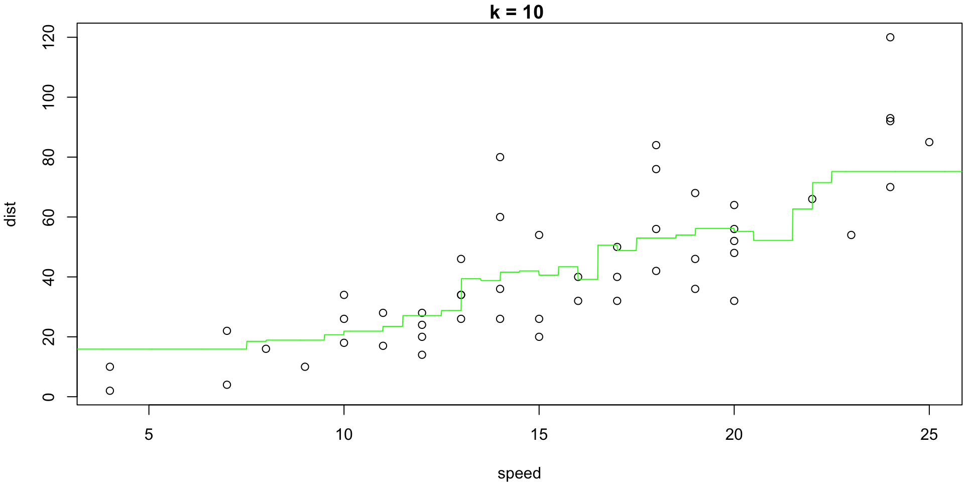
k = 10

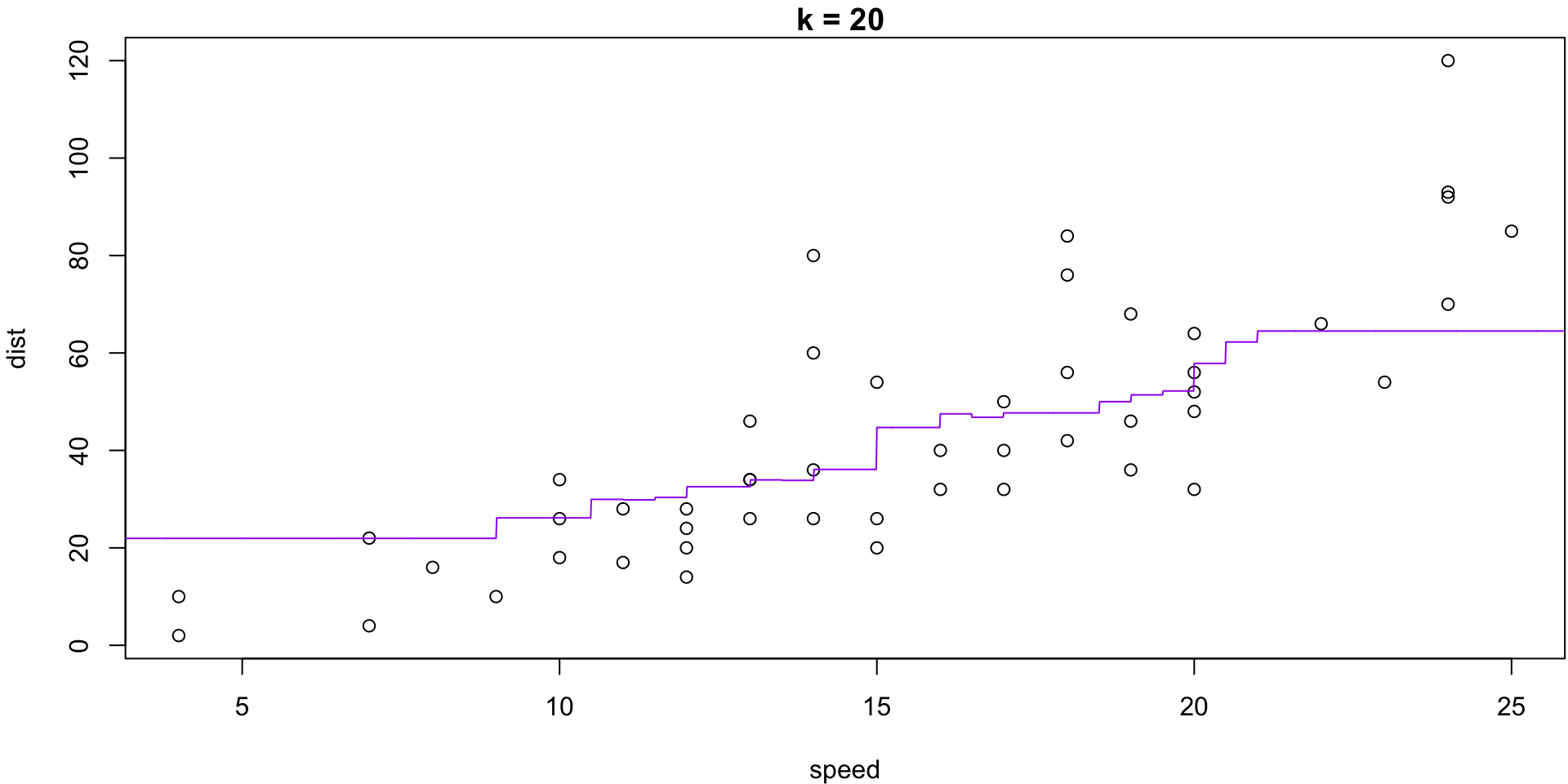
k = 20

not flexible enough

k = 2 (winner)

• To flexible?
• speed is quite discretized
• best model is to just average the y’s at each vertical collection of points
• for jittered x i suspect a higher k would be selected

Comparing Models

• Not only can we select k using CV, but we can furthermore compare that best KNNreg model’s predictive performance with any other potential model.

• Since CV estimates the MSE, there’s no reason we cannot provide that estimate in the context of, say, simple linear regression…

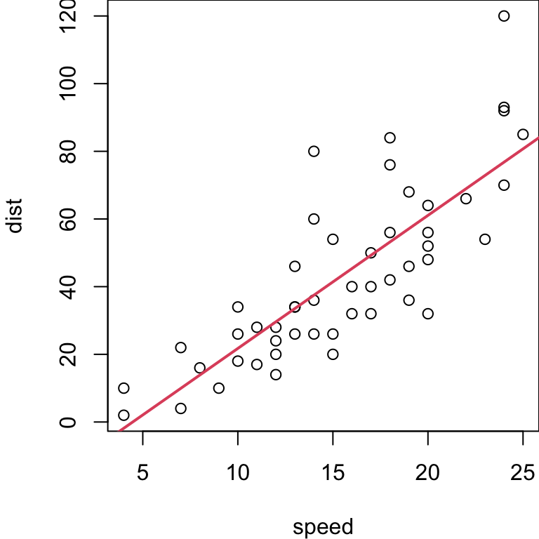
Cars example (regression)

Car data, simple linear regression on full sample

cars.line <- lm(dist~speed)
summary(cars.line)

...
Call:
lm(formula = dist ~ speed)

Coefficients:
            Estimate Std. Error t value Pr(>|t|)    
(Intercept) -17.5791     6.7584  -2.601   0.0123 *  
speed         3.9324     0.4155   9.464 1.49e-12 ***
---
Signif. codes:  0 '***' 0.001 '**' 0.01 '*' 0.05 '.' 0.1 ' ' 1

Residual standard error: 15.38 on 48 degrees of freedom
Multiple R-squared:  0.6511,    Adjusted R-squared:  0.6438 
F-statistic: 89.57 on 1 and 48 DF,  p-value: 1.49e-12
...

Regression MSE estimate

• Under the inferential assumptions for SLR, we have a theoretical (unbiased) estimate of the test MSE via \[ \hat{\text{MSE}} = \frac{\text{RSS}}{n-2} = \frac{\sum (y_i - f(x_i))^2}{n-2}\]

• For the cars data, that gives us: \(\frac{11353.52}{48}= 236.53\)

• In this case k = 2 KNN model gets a CV MSE estimate of 178.54 hence is suggested as the better model.

Assuming all our diagnostics hold and we’re willing to make those inferential assumptions,

LOOCV Regression Shortcut

• While we could compare these estimates of MSE directly, we could go one step further and get the CV estimate for MSE by applying LOOCV to the linear model!

• Notably, there is a mathematical shortcut for LOOCV with the least squares linear or polynomial regression that calculate \(CV_{(n)}\) using a single fit!

• The details of this shortcut are discussed in Section 5.1.2 of the ILSR textbook (we won’t go over them here).

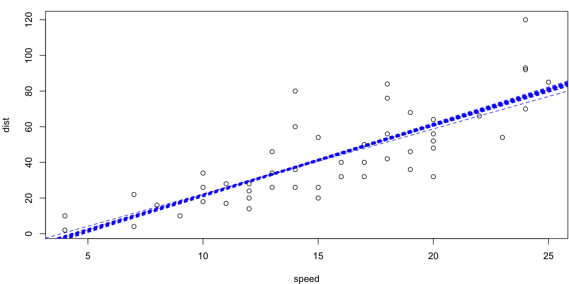
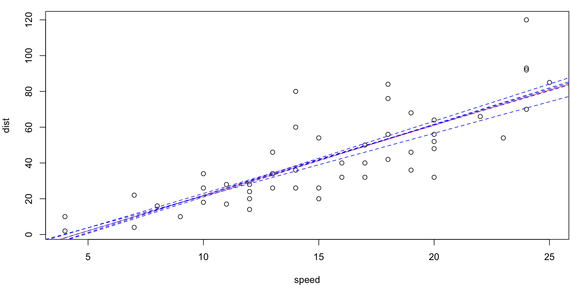
LOO Regression Animation

LOO regression fits

Plots the \(n\) (highly correlated) LOOCV regression fits produce a cross-validated estimates MSE = \(CV_{(n)} = 246.405416\)

only one blue line out of place for that higher leverage point

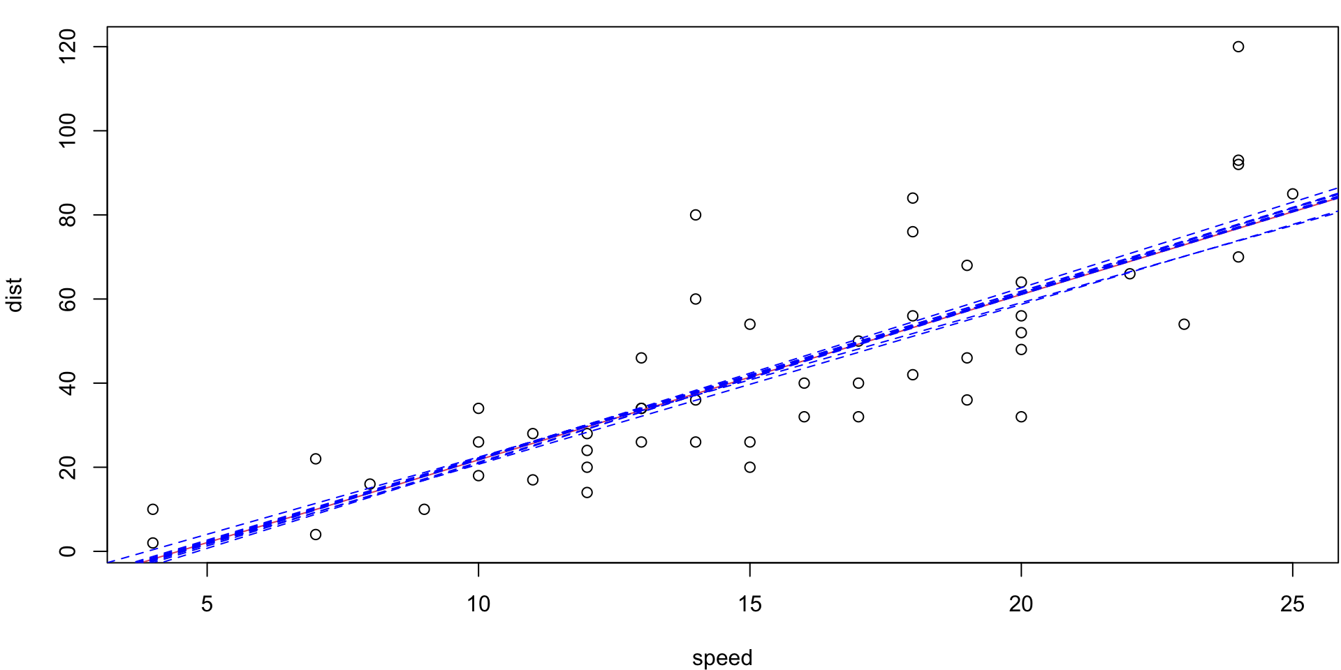
5-fold CV Animation

• this estimate would be different if we ran it again (unlike LOO)
• more variation in the lines and only have 5 of them
• less correlation in the lines give less variance for MSE
• if we did this again and agin on new data, the estimate of MSE would have higher variance for LOOCV than k-fold

5-fold estimates MSE as \(CV_{(5)} = 254.0391118\)

• compared to LOOCV estimate of 246 (low bias high variance)
• similar value (higher bias lower variance)

10-fold CV Animation

now we have 10 validation sets (with 5 obs in each) n=50

10-fold estimates MSE as \(CV_{(10)} = 243.7798735\)

Summary

\(k\)	\(CV_{(k)}\)
5	254.04
10	243.78
\(n\) (LOOCV)	246.41

• LOOCV fits are highly correlated (almost identical)
• The smaller correlatiaon between the fits in k-fold results in less variability in the MSE estimate.
• As stated before, 5- or 10- fold CV tend to produce more accurate estimates of test error than LOOCV (which tends to overestimate).

Wine example

• We now consider the wine data set from the pgmm package

• 27 measurements on 178 samples of red wine.

• Samples originate from the same region of Italy (Piedmont), but are of different varietals (Barolo, Barbera, Grignolino).

• We can do KNN classification, using LOOCV¹ to choose k, the number of neighbours…

1. We will use knn from the class package and hard-code LOOCV (R script posted to Canvas)

Best k

In this case the minimum is at k = 8

source code at lectures/code/13/wine.R

Wine Example

We can provide a cross-validated classification table,

	Predicted
	1	2	3
Barolo	52	3	2
Grignolino	2	59	11
Barbera	5	9	35

or LOOCV Error …

\[ \begin{align} CV_{(n)} &= \frac{1}{n} \sum_i^n \text{Err}_i\\ & = \frac{1}{n} \sum_i^n I(y_i \neq \hat y_i)\\ & = \frac{32}{178} = 0.18 \end{align} \]

… or cross-validated versions of any of our other classification performance indices exist!

prime you for next lecture - not that the model we used here was the \(k\)=8 group model fitted to the entire data set.

Standard Errors

• More generally: \(CV_K = \sum_{k=1}^K \frac{n_k}{n} \text{Err}_k\)

• In addition to computing \(CV_K\) estimate of the error rate, we can also estimate standard deviation of \(CV_K\).

• The estimated standard deviation of \(CV_K\) is given by:

\[\begin{equation} \hat{\text{SE}}(CV_K) = \sqrt{ \sum_{k=1}^{K} \left(\text{Err}_k - \overline{\text{Err}_k}\right)^2/ (K-1)} \end{equation}\]

• \(SE(CV_{(K)}\) estimate is a measure that quantifies the variability of the CV estimate itself.
• tells how reliable and stable the performance evaluation of a predictive model is when using cross-validation.
• Err\(k\) overlaps with Err\(j\) cuz they share some training samples
• nevertheless people use it anywya

While this is a useful estimate, but strictly speaking, not quite valid since observations are not independent

Final Remark

• Now we have \(n\) different fits of the model, which model should we report?

None of them

• While CV is used to help select a model, the actual reported model would be the one run with all the data.

• That is, we would need to run knn() with k = 8 on the full data set with no observations removed.