Data 311: Machine Learning

Lecture 7: Bayes Classifier, KNN Classification and Discriminant Analaysis

Dr. Irene Vrbik

University of British Columbia Okanagan

Introduction

• Last class we introduced the logistic regression model used for binary classification¹. Therein we modeled:

  \[ \Pr( \text{class} = 1 \mid \text{data}) \]

• Today we will continue with classification methods:

  • Bayes Classifier
  • KNN Classification
  • [LDA] Linear Discriminant Analysis

• we saw the confusion matrix and metrics built off of it like error rate, precision, specificity and F1

• talked about how the multinomial can be extend it to >2 classes

• From previous lectures, we know that the Bayes classifier has the lowest possible error rate (assuming the model is correctly specified)

• Remember, the Bayes classifier assigned observation \(x\) to class \(k\) for which \(P(Y = k \mid X = x)\) — the conditional distribution of the response \(Y\), given the predictor(s) \(X\) — is the largest.

• We have already seen a couple methods for obtaining estimates for \(P(Y = k \mid X = x) := p_k(x)\) (shorthand notation used in the ISLR2 textbook)

1. i.e. our categorical response variable \(Y\) is either a 0 or a 1.

Test Error Rate

• A good classifier is one for which the test error is smallest.
• The test error rate associated with a set of test observations of the form (\(x_0, y_0\)) is given by

\[\begin{equation} \text{Avg}(I(y_0 \neq \hat y_0)) \end{equation}\]

where \(\hat y_0\) is the predicted class label that results from applying the classifier to the test observation with predictor \(x_0\).

this concept is similar to \(MSE_{test}\)

Bayes Classifier

• “Bayes classifier” is a general concept that refers to any classifier that makes predictions based on Bayes theorem

• A Bayes classifier calculates the probability of a particular class given a set of features and then selects the class with the highest probability as the prediction.

• It can be shown¹ that the Bayes Classifier minimizes the testing error given on the previous page.

proof outside the scope of the course - In other words, if we assign predictions to the class with the highest probability, a bayes classifier will make the fewest mistakes on average.

• The “Naive Bayes classifier” is a specific type of Bayes classifier.

1. though the proof is outside the scope of this course

Bayes Theorem

Bayes’ theorem relates conditional probabilities.

\[\begin{equation} P(A|B) = \frac{P(B|A) \cdot P(A)}{P(B)} \end{equation}\]

• \(P(A|B)\) is the conditional probability of event A occurring given that event B has occurred.

• \(P(B|A)\) is the conditional probability of event B occurring given that event A has occurred.

• \(P(A)\) is the marginal probability of event A

• \(P(B)\) is the marginal probability of event B

Definition

• The Bayes classifier assigns each observation to the most likely class, given its predictor/input values (i.e. \(X\)s ).

• That is, for some predictor vector \(x_0=(x_{01}, x_{02}, \ldots, x_{0p})\) we should assign the class \(j\) where the following conditional probability is maximized: \[P(Y=j \mid X=x_0)\]

Note that this is a conditional probability: it is the probability that \(Y = j\), given the observed predictor vector \(x_0\).

In a two-class problem where there are only two possible response values, say class 1 or class 2, the Bayes classifier corresponds to predicting class one if \(P(Y = 1 \mid X = x_0) > 0.5\), and class two otherwise.

Bayes Decision Boundary Definition

For the two class problem the Bayesian decision boundary is defined as the line where

\[P(Y=1 \mid X=x_0) = P(Y=2 \mid X=x_0)\]

This boundary separates the feature space into two decision regions:

• Region 1 points for which \(P(Y = 1 \mid X = x_0) > 0.5\) and are assigned to class 1
• Region 2 points for which \(P(Y = 1 \mid X = x_0) < 0.5\) and are assigned to class 2

this idea can be extended to more classes

Bayes Classifier Example

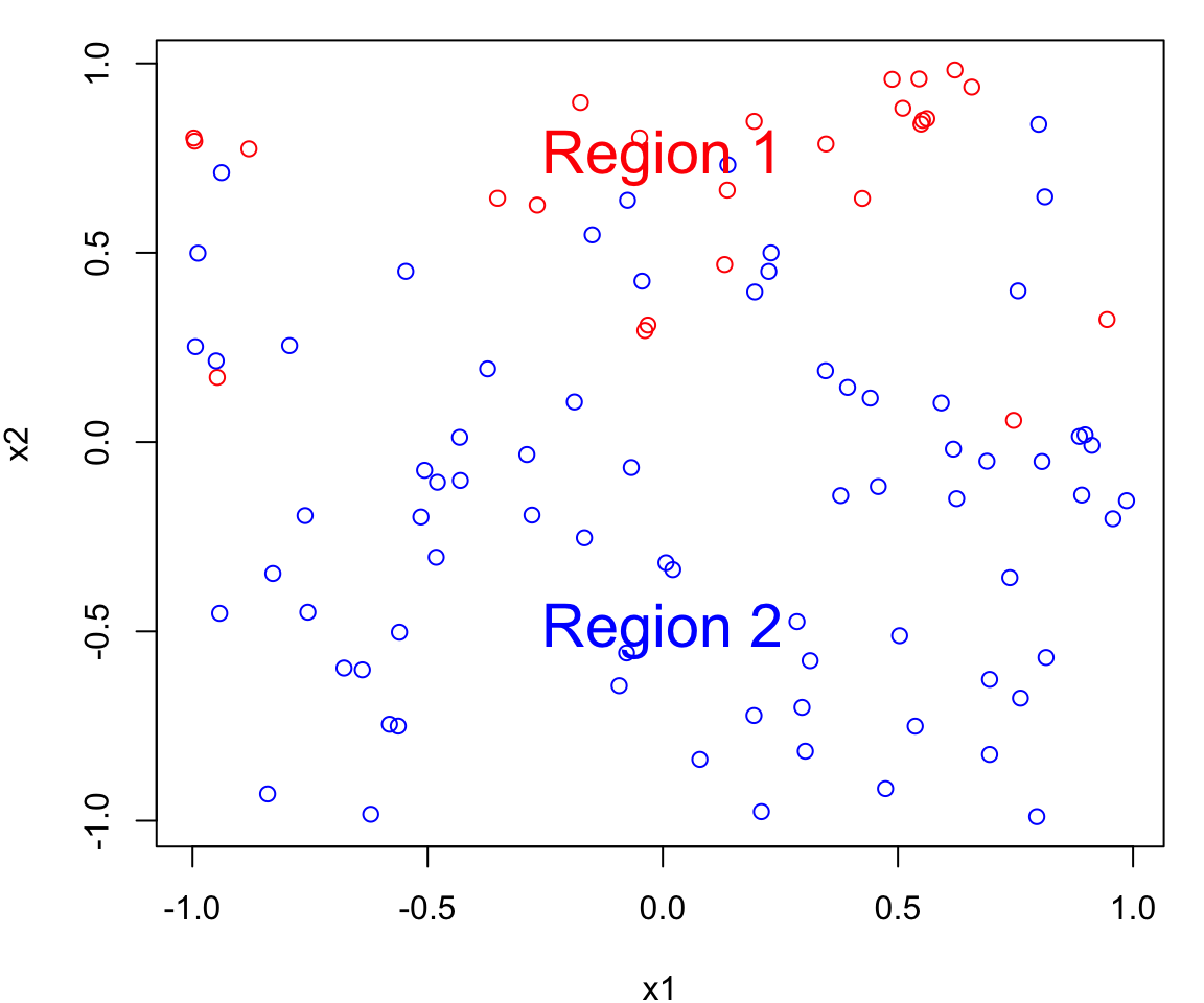
• Let’s simulate a data set with of two continuous predictors \(X_1\) and \(X_2\); both uniformly distributed from \([-1, 1]\).

• We create two classes:

  • a red group (corresponding to \(Y=0\)) and
  • a blue group (corresponding to \(Y=1\))

• To generate the class assignment we will only using \(X_2\).

• That is \(X_1\) is represents a useless predictor.

Class generation

We will assign an observation to a class based on the following:

If \(x_2 > 0\)

\[\begin{align} P(Y = 0 \mid X_2 = x_2) &= x_2\\ P(Y = 1 \mid X_2 = x_2) &= 1 - x_2 \end{align}\]

If \(x_2 \leq 0\)

\[\begin{align} P(Y = 0 \mid X_2 = x_2) &= 0\\ P(Y = 1 \mid X_2 = x_2) &= 1 \end{align}\]

Take the compliment of those probabilities to show the probabilities for belonging to the blue group:

Notice that \(x_{1i}\) does not provide any information about the class.

• The red and blue circles correspond to training observations that belong to two different classes.
• For each value of X1 and X2, there is a different probability of the response being red or blue.
• Since this is simulated data, we know how the data were generated and we can calculate the conditional probabilities for each value of X1 and X2.

• Any point above the dotted line reflects the set of points for which Pr(Y = red|X) is greater than 50%,
• while and point below the blue shaded region indicates the set of points for which the probability is below 50%.
• The purple dashed line represents the points where the probability is exactly 50%.

• The purple dashed line is called the Bayes decision boundary.
• The Bayes classifier’s prediction is determined by the Bayes decision boundary; an observation that falls on the red side of the boundary will be assigned to the red class, and similarly an observation on the blue side of the boundary will be assigned to the blue class.

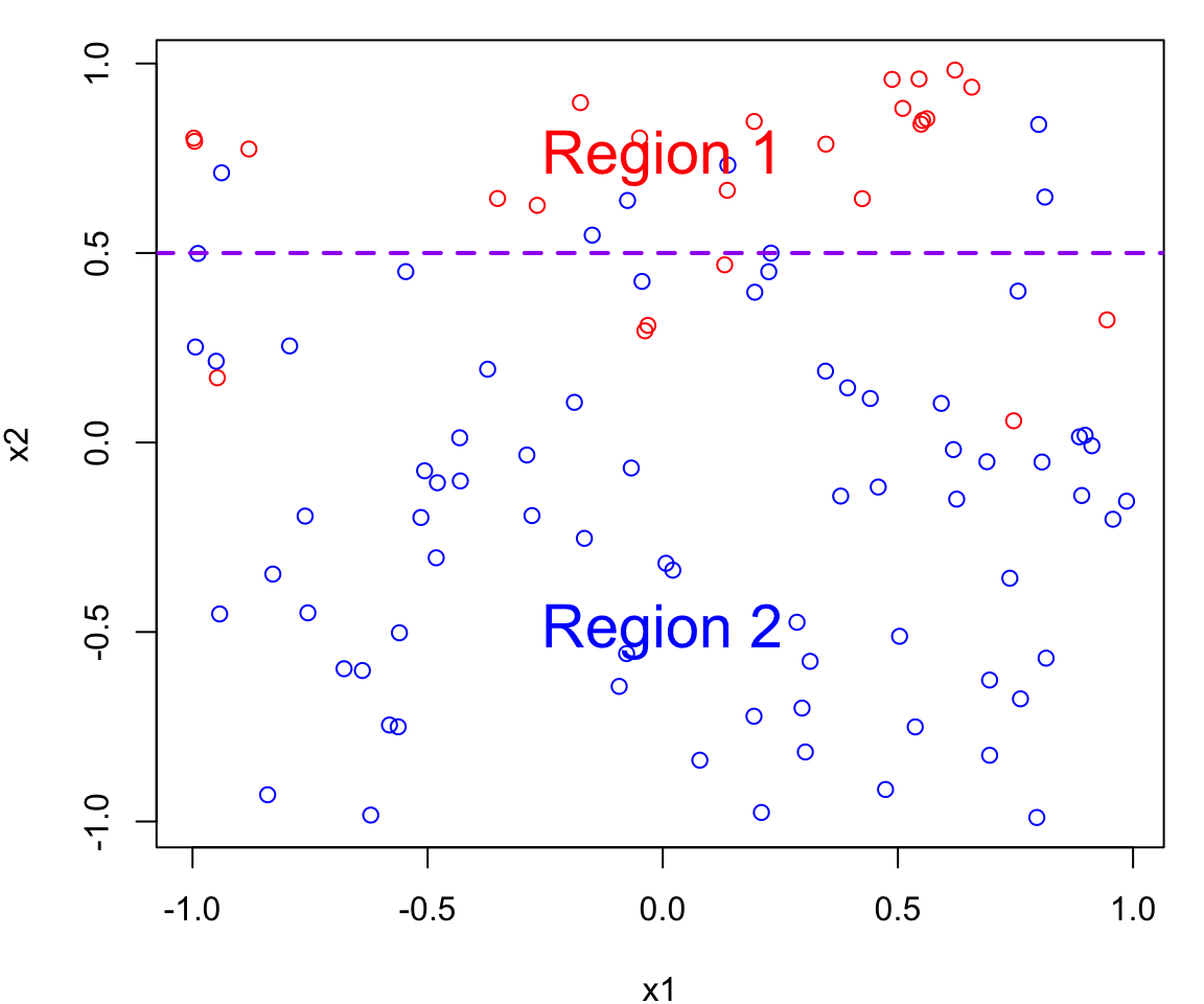
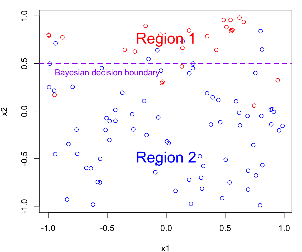
Bayes Decision Boundary

• The Bayes decision boundary represents the dividing line in the feature space (i.e. in terms of \(X\)s) that determines how data points are classified into different classes.

• In our case data points below the decision boundary (Region 1) are classified as red, while data points above the decision boundary (Region 2) are classified as blue

• Note that errors are still going to be made using this classifier since the process is random (points near the boundary are sometimes going to red in Region 2 and sometimes blue in Region 1)

heres its a line in higher dimension it can be a surface and we’ll see how it can take more complicated forms (eg. islands) later

Optimal Boundary

• The Bayes decision boundary represents the optimal decision boundary because it’s based on the true underlying probability distributions of the data.

• In other words, the Bayes decision boundary is going to make fewer mistakes than any other classifier you will come up with.

Note

In practice, these distributions are often unknown and need to be estimated from data, which can introduce uncertainty.

Bayes Error Rate

On average, Bayes classifier will yield the lowest possible test error rate given by the following expectation (averages the probability over all possible values of \(X\)) \[1-E\left( \max_j P(Y=j \mid X) \right)\]

The above is called the Bayes error rate which represents the minimum possible error rate that any classifier can achieve for a given classification problem.

• Our bayes error is greater than zero, because there is classes overlap in the true population so maxj Pr(Y = j|X = x0) < 1 for some values of \(x_0\).
• Notice if the is no error than the prob inside the () is 1 and the error is 0. But since there is some stochasic behaviour in our data Bayes error > 0
• You can think of this error as overlaping classes in your population 1 Problem: in practice we won’t know the conditional probability \(P(Y=j \mid X)\)!

The Bayes error rate is analogous to the irreducible error, discussed in previous lectures.

From simulations to real data

• In theory we would always like to predict qualitative responses using the Bayes classifier.
• But for real data, we do not know the conditional distribution of \(Y\) given \(X\), and so computing the Bayes classifier is impossible.
• Therefore, the Bayes classifier serves as an unattainable gold standard against which to compare other methods.

Classification Algorithms

• Many approaches attempt to estimate the conditional distribution of \(Y\) given \(X\), and then classify a given observation to the class with highest estimated probability.

• For example, Logisitic Regression modeled

  \[ \Pr(Y_i = 1 \mid X_i = x_i) \tag{1}\]

  and \(X_i\) is assigned class 1 if this probability is \(\geq 0.5\).

• Another example is the \(K\)-nearest neighbors (KNN) \(\dots\)

KNN Classification

• Given a positive integer \(K\) and a test observation \(x_0\), the KNN classifier first identifies the \(K\) points in the training data that are closest to \(x_0\), represented by \(\mathcal{N}_0\).

• For each class \(j\), find \[\begin{equation} P(Y=j \mid X=x_0) \approx \frac{1}{K} \sum_{i \in N_0} I(y_i = j) \end{equation}\]

• Assign observation \(x_0\) to the class (\(j\)) for which the above probability is largest; “ties” are typical broken at random (i.e. a coin toss)

Very intuitive, we look at the \(k\) closest values to a new point and see if they are mostly red or blue. Whichever class has the majority is the class where the object gets assigned

• This algorithm is similar to the KNN regression, only now, rather than averaging continuous \(y\) values, we are counting the number of neighbors that belong to each class.

• The majority class among the \(K\)-nearest neighbors is chosen as the predicted class for the new data point.

in R

To demo knn classification we will be using the knn function from the class package performs (other alternatives exist)

library("class")
knn(train, test, cl, k)

• train matrix or data frame of training set cases.
• test matrix or data frame of test set cases.
• cl factor of true classifications of training set
• k number of neighbours considered.

k - how to choose?

As indicated in the documentation “ties” are broken at random.

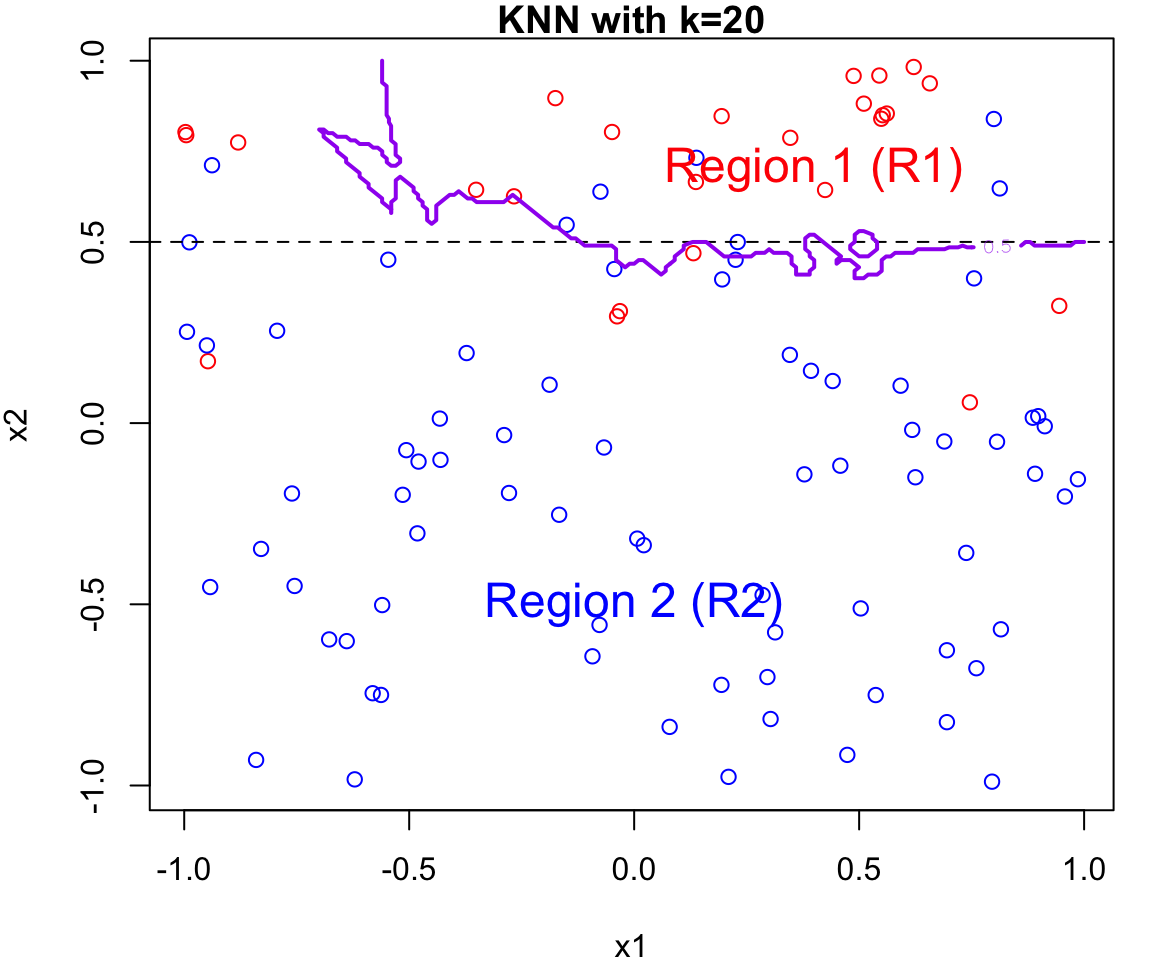
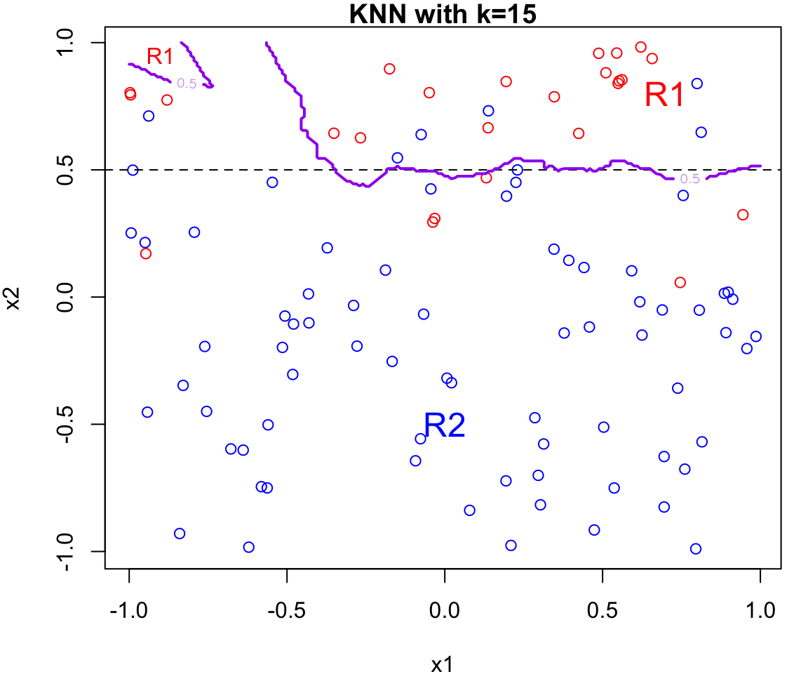
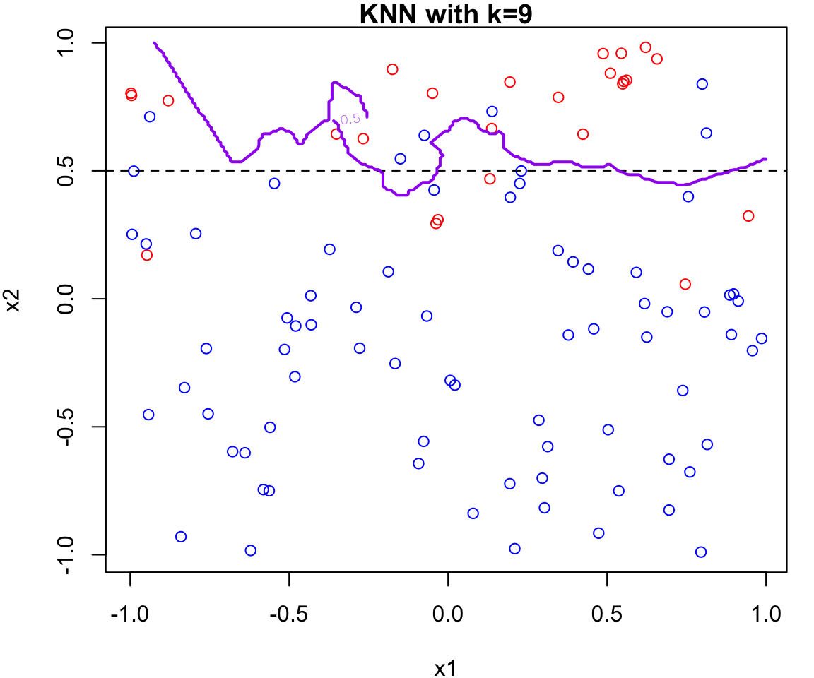
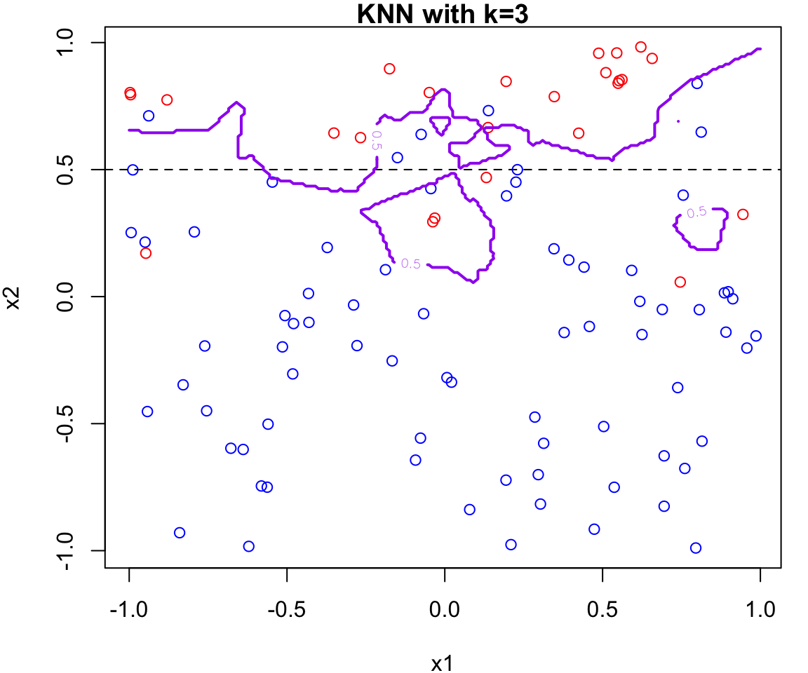
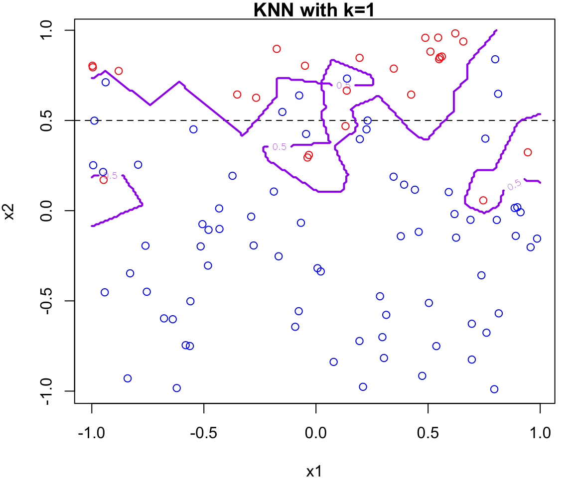
k Nearest Neighbours Example

• Let’s apply this algorithm to the simulated data considered previously.

• More specifically, we will fit knn for \(k = 20, 15, 9, 3\) and \(1\)

• Fair warning that the decision boundary and decision regions will not be as clear cut as our previous example.

• We will assess the error rate for each (code presented in lab)

An great interactive demo can be view here

So rather than a boundary like you get these little islands

Choosing k

• A key component of a “good” KNN classifier is determined by how we choose \(k\), the number of nearest neighbours.

• \(k\) in a user-defined input which we can set anywhere from 1 to \(n\) (the number of points in our training set)

  • Choose odd k to avoid ties in binary classification.

  • Use cross-validation to find the optimal k value for your dataset. (more on this later in the course).

Question What would happen if \(k\) was set equal to \(n\)?

• every observation would get assigned to the most prevalent class in our training set.
• Since there are more red points than blue points, all future observations will get predicted to the red class.
• when \(k=n\) we predict the most common class (over simplistic)

Discuss some general rules of thumb for small/large \(k\)?

• Larger values of \(k\) tend to predict most commonly occurring class
• As \(k\) increase this model increase in simplicity and we get more BIAS
• As \(k\) decrease we tend to get overly flexible models, ie overfit. Boundaries change significantly with different training sets and the variance increases!
• What is this the product of? Bias-Variance tradeoff!
• You will see the same patter in the training (decreasing) and testing error (U shape); not shown here go to book.

iClicker: small neighborhood

What happens to the decision boundary in KNN when the value of \(k\) is too small (e.g., k=1)?

1. The model becomes more robust to noise
2. The decision boundary becomes smoother
3. The model becomes more sensitive to noise
4. The model becomes less flexible

Correct answer: C.

Some explanation

iClicker

k related to bias-variance

In KNN, increasing \(k\) tends to:

1. Increase bias and decrease variance
2. Increase both bias and variance
3. Decrease both bias and variance
4. Decrease bias and increase variance

Correct answer: A. Increase bias and decrease variance

Recap

To estimate the conditional distribution of \(Y\) given \(X\),

• KNN did this using a “voting” system with its nearest neighbours \(\Pr(Y=j \mid \boldsymbol x) \approx \frac{1}{K} \sum_{i \in N_0} I(y_i = j)\)

• Logistic regression uses the logistic function, e.g. \[\Pr(Y = 1 \mid \boldsymbol x) = \frac{e^{\beta_0 + \beta_1x}}{1 + e^{\beta_0 + \beta_1x}}\]

Let’s discuss linear and quadratic discriminant analysis as alternative methods for approximating the conditional distribution of \(Y\) given \(X\) \(\dots\)

WHY logistic regression not natural in the MV setting

• When there is substantial separation between the two classes, the parameter estimates for the logistic regression model are surprisingly unstable. The methods that we consider in this section do not suffer from this problem.
• If the distribution of the predictors X is approximation normal in each class and the sample size is small this may be more accurate than Log reg

Bayes Theorem

\[ \Pr(Y = k \mid \boldsymbol x) = \frac{\Pr(\boldsymbol x \mid Y = k)\cdot \Pr(Y = j)}{\sum_{j} \Pr(\boldsymbol x \mid Y = k)\cdot \Pr(Y = k)} \]

• we can assume some model for \(\Pr(\boldsymbol x \mid Y = k) \sim f_k(\boldsymbol x)\) (e.g. Gaussian)

• \(\Pr(Y=k)\) is the prior, denoted \(\pi_k\). It represents the prior probability of observation \(\boldsymbol x\) belonging to class \(k\)

The denom is not important since that will be the same for all classes

so we assign observatiosn to the whichever class gives the highest denominator

to match the textbook we will use \(k\) to index the \(K\) classes now

Posterior Probabilities

Then Bayes’ theorem states that

\[\begin{equation} \Pr(Y = k \mid X = x) = \frac{\pi_k f_k(x)}{\sum_{l=1}^{K} \pi_l f_l(x)} \end{equation}\]

This represents the posterior probability that an observation \(X = x\) belongs to the \(k\)th class.

• \(\pi_k\) is the prior probability that an observation \(X= x\) belongs to the \(k\)th class
• That is, it is the probability that the observation belongs to the kth class, given the predictor value for that observation.
• now let’s plug in the Gaussian distribution for \(f_k(x)\)
• The prior in discriminant analysis represents the initial assumption about how likely each class is before observing any data.

To estimate \(p_k(x)\), and thereby approximate the Bayes classifier, we can need to estimate the \(\pi_k\)s and \(f_k(x)\).

• estimating πk is easy if we have a random sample from the population: we simply compute the fraction of the training observations that belong to the kth class.
• However, estimating the density function fk(x) is much more challenging.
• As we will see, to estimate fk(x), we will typically have to make some simplifying assumptions.

We will abbreviate this to \(p_k(x) = \Pr(Y = k|X = x)\)

Discriminant Analysis

We assume a normal (Gaussian) distributions with mean vector \(\boldsymbol{\mu}_k\) and covariance matrix \(\boldsymbol{\Sigma}_k\) for each class

\[f_k(\mathbf x) = \frac{1}{(2\pi)^{p/2}|\boldsymbol{\Sigma}_k|^{1/2}} e^{-\frac{1}{2}(\mathbf{x}-\boldsymbol{\mu}_k)^T\boldsymbol{\Sigma}_k^{-1}(\mathbf{x}-\boldsymbol{\mu}_k)}\]

Important

Depending on our assumptions on \(f_k(\boldsymbol x)\), this leads to linear discriminant analysis (LDA) or quadratic discriminant analysis (QDA).

Here the approach is to model the distribution of \(X\) in each of the classes separately, and then use Bayes’ theorem to flip things around and obtain \(\Pr(Y |X)\).

This approach is quite general, and other distributions can be used as well.

Which class does the new point as indicated by the star belong to?

To answer this, it might be useful to talk about a decision boundary.

This will depend on our priors and parameters.

to answer this we need the priors and the likelihood.

Once we have that we can multiply them together to get the probability.

we will need to estimate these using the data.

Generative Models for Classification

• For simplicity, let’s suppose we have two classes, that is \(Y\) can take on two possible values \(K = 1\) or \(K = 2\)

• Let \(f_k(X) \equiv \Pr(X\mid Y = k)\) denote the pdf of \(X\) for an observation that comes from the \(k\)th class.

• Let \(\pi_k\) represent the overall or prior probability that a randomly chosen observation comes from the \(k\)th class.

In other words, \(f_k(x)\) is relatively large if there is a high probability that an observation in the \(k\)th class has \(X \approx x\), and \(f_k(x)\) is small if it is very unlikely that an observation in the \(k\)th class has \(X \approx x\).

LDA for one predictor

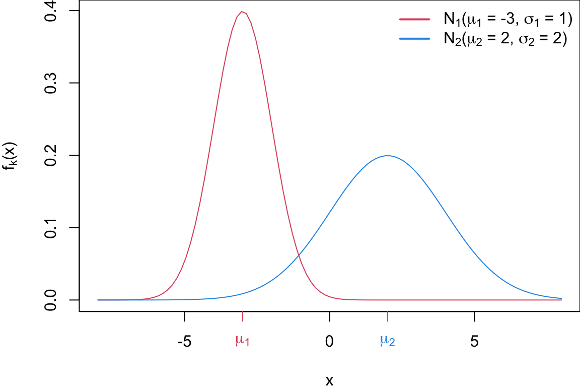
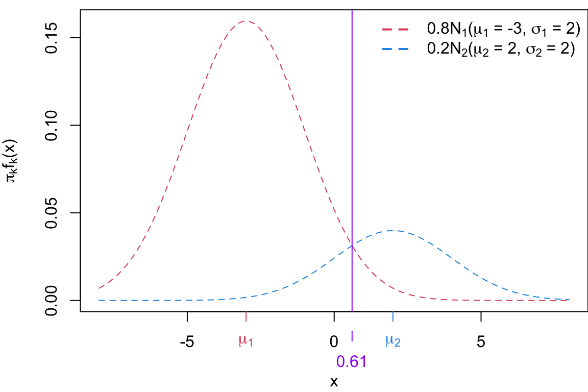
For simplicity let’s assume \(x\) is univariate so that \(f_k(x)\) be the is univariate Normal distribution with mean \(\mu_k\) and \(\sigma_k^2\) for an observation from the \(k\)th class.

\[\begin{equation} f_k(x; \mu_k, \sigma_k) = \frac{1}{\sqrt{2\pi}\sigma_k} e^{-\frac{(x-\mu_k)^2}{2\sigma_k^2}} \end{equation}\]

Before we estimate \(f_k(x)\), we will first make some assumptions about its form.

The \(\pi\) without a subscript is the constant 3.14159….

Univariate Normal Distribution

Sticking with univariate for now, suppose each group is normally distributed with different means and variances

\[\begin{align*} f_1(x) &\sim N(\mu_1, \sigma_1^2)\\ f_2(x) &\sim N(\mu_2, \sigma_2^2) \end{align*}\]

While discuss this method in 2-class univariate setting these concepts can be extended to the multivariate distributions with \(>2\) classes.

Plot of two univariate normals

The red curve represents \(f_1 = N(\mu_1 = -3, \sigma_1 = 1)\), and the blue curve represents \(f_2 = N(\mu_2 = 2, \sigma_2 = 2)\).

par(mar = c(3.9,4.1,0,0))
pi1 = 0.6
pi2 = 1 - pi1
curve(dnorm(x, mean = mean1, sd = sd1), col = 2, from = -8, 8, ylab = expression(paste(pi[k]*f[k]*"("* x *")")), lty = 1)
curve(dnorm(x, mean = mean2 , sd = sd2), col = 4, add = TRUE, lty = 1)
gmm <- function(x, pis, mus, sigs){
  pis[1]*dnorm(x, mean = mus[1], sd = sigs[1]) +
    pis[2]*dnorm(x, mean = mus[2], sd = sigs[2]) 
}    
# curve(gmm(x, c(pi1, pi2), c(mean1, mean2), c(sd1, sd2)), col = 3, add = TRUE)
 curve(pi1*dnorm(x, mean = mean1, sd = sd1), col = 2, from = -8, 8, ylab = expression(paste(pi[k]*f[k]*"("* x *")")), lty = 2, add = TRUE)
 curve(pi2*dnorm(x, mean = mean2 , sd = sd2), col = 4, add = TRUE, lty = 2)
axis(1, at=mean1, labels = expression(mu[1]), col=2, col.axis=2)
axis(1, at=mean2, labels = expression(mu[2]), col=4, col.axis=4)        
ltext <- c(bquote(N[1]*"("*mu[1] *" = "* .(mean1)*", "*sigma[1] *" = "* .(sd1) * ")"),
           bquote(N[2]*"("*mu[2] *" = "* .(mean2)*", "*sigma[2] *" = "* .(sd2)* ")"),
           bquote(pi[1] *" = "* .(pi1)*", "*pi[2] *" = "* .(pi2)))
    legend("topright", lwd= 2, col = c(2,4,NA), 
           legend = ltext, bty = "n")

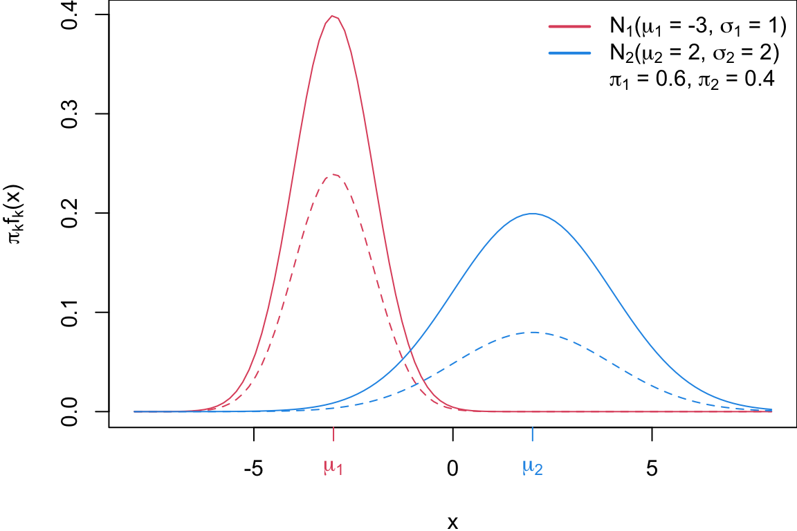
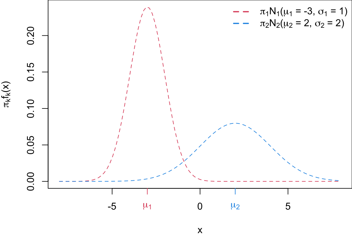
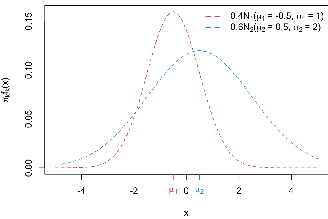
The solid lines denote \(f_k\), the dashed lines show \(\pi_k * f_k\), i.e. the distributions weighted by their class probabilities \(\pi_1 = 0.6\) and \(\pi_2 = 0.4\).

• we need to find the decision boundary
• We are going to classify a new point according to which numerator is the biggest

Building a classifier

We classify new points according to whichever numerator \((\pi_k f_k(x))\) is the highest.

Question: where would that decision boundary be on this picture?

• we need to find the decision boundary
• We are going to classify a new point according to which numerator is the biggest

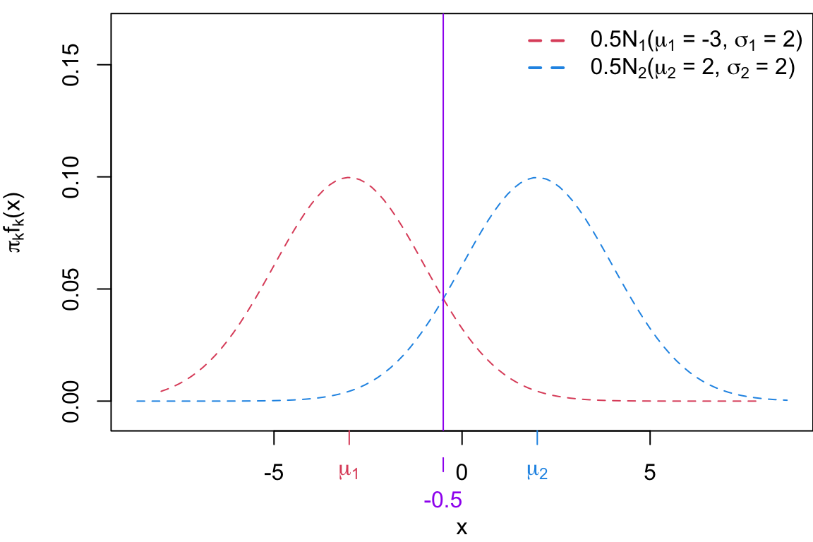
Case 1

Case 1: \(\sigma_1 = \sigma_2\) and \(\pi_1 = \pi_2\) If the class variances and priors are equal, we have a linear decision boundary which is simply the average of the means: \(x = \frac{\mu_1 + \mu_2}{2}\)

when we two groups with equal varianace and prior probabilities, the decision boundary is just the average of the two means (as you might have guessed and we can prove using math)

Case 2

Case 2: \(\sigma_1 = \sigma_2\) and \(\pi_1 \neq \pi_2\) If the class variances are samle and the priors are different, the decision boundary is still linear but shifted toward the class with the lower prior probability (the less likely class), i.e. \(x = \frac{\mu_1 + \mu_2}{2} + \frac{\sigma^2}{\mu_1 - \mu_2} \log \left( \frac{\pi_1}{\pi_2} \right)\)

• the boundary is where they intersect but it’s shifted to the right, which makes sense …
• there are more group 1 class than group 2 so the prior probability of belonging to class one is higher.
• the bigger prior has bumped up the rotted red curve and moved the decision boundary to the right
• there are more reds so all else being equal we are going to make less mistakes if we classify more observations to the red group.

Case 3

Case 3: \(\sigma_1 \neq \sigma_2\) and \(\pi_1 \neq \pi_2\) If the class variances are samle and the priors are different, the decision boundary is non-linear (quadratic).

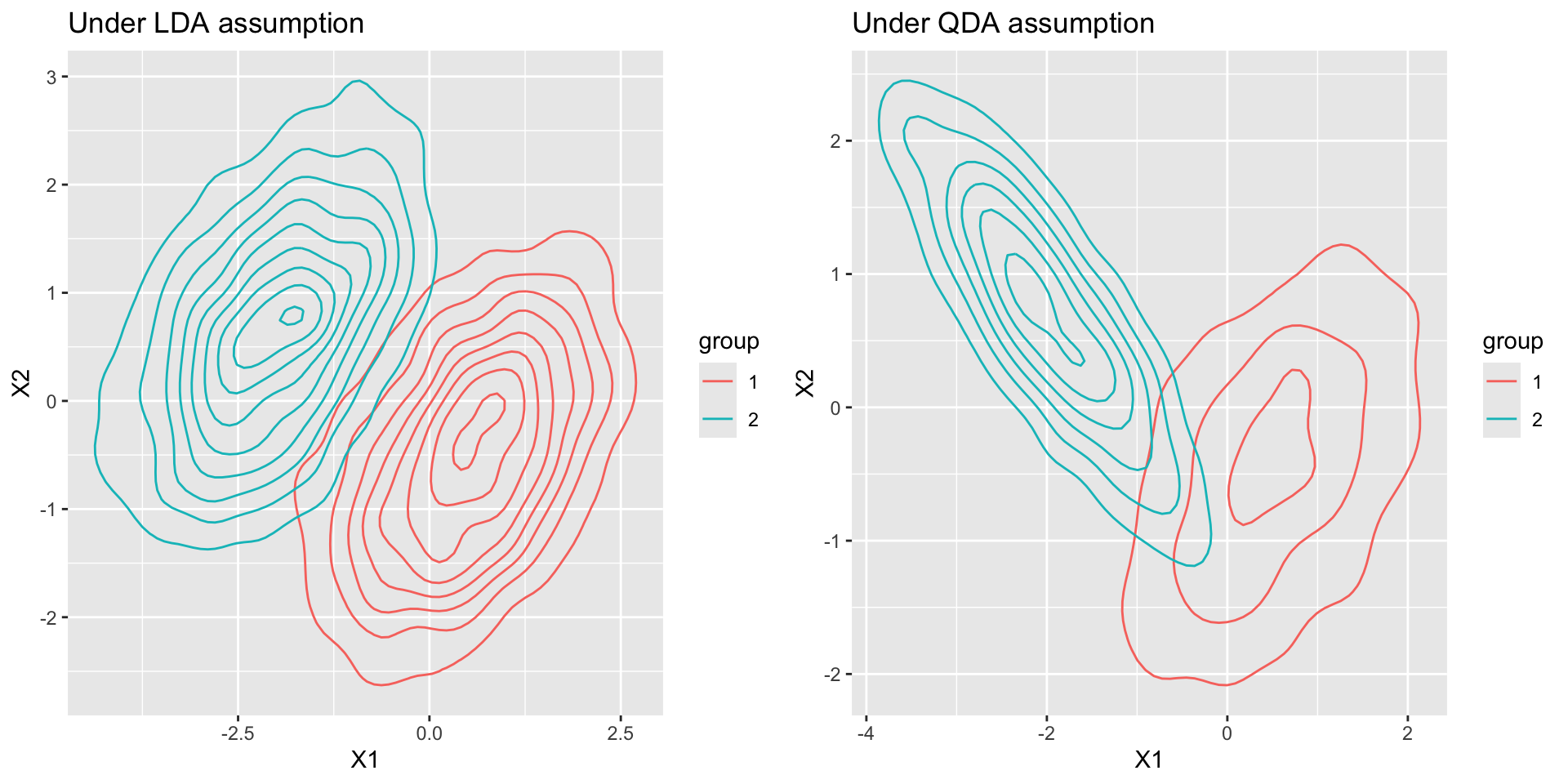
LDA vs QDA Assumptions

• Linear Discriminant Analysis (LDA) assumes that the variances of all classes are equal, i.e., \(\sigma_1 = \sigma_2 = \sigma\), where \(\sigma\) represents the common variance.

• When we relax this assumption and allow for different variances between the groups, we get Quadratic Discriminant Analysis (QDA). In QDA, we have \(\sigma_1 \neq \sigma_2\), meaning the variances differ across the classes.

you might as why we need LDA? it just produces a linear boundary in the same way logistic regression does, but it’s a little different.

For simplicity, we will sometimes assume equal priors (\(\pi_1 = \pi_2\)). If this assumption is relaxed (i.e., when the priors are unequal), the decision boundary shifts toward the class that is less likely.

LDA decision boundary

Since we’re dealing with two classes, we can set the decision boundary where \(p_1(x) = p_2(x)\)

Assumption \(\sigma_1 = \sigma_2\) (but the \(\pi_k\)s will vary)

\[\begin{align} \frac{\pi_1 f_1(x)}{\sum_{l=1}^{K} \pi_l f_l(x)} &= \frac{\pi_2 f_2(x)}{\sum_{l=1}^{K} \pi_l f_l(x)} \\ \frac{\pi_1}{\sqrt{2\pi}\sigma} e^{-\frac{(x-\mu_1)^2}{2\sigma^2}} &= \frac{\pi_2}{\sqrt{2\pi}\sigma} e^{-\frac{(x-\mu_2)^2}{2\sigma^2}}\\ \vdots \end{align}\]

denoms are common

Canceling the common terms, and taking the logarithm of both sides:

\[ \log(\pi_1) - \frac{(x - \mu_1)^2}{2 \sigma^2} = \log(\pi_2) - \frac{(x - \mu_2)^2}{2 \sigma^2} \]

Expanding the quadratic terms:

\[ \log(\pi_1) - \frac{x^2 - 2x \mu_1 + \mu_1^2}{2 \sigma^2} = \log(\pi_2) - \frac{x^2 - 2x \mu_2 + \mu_2^2}{2 \sigma^2} \]

Simplifying both sides:

\[ \log(\pi_1) + \frac{2x \mu_1 - \mu_1^2}{2 \sigma^2} = \log(\pi_2) + \frac{2x \mu_2 - \mu_2^2}{2 \sigma^2} \]

If the left-hand side (LHS) is greater than the right-hand side (RHS), the observation is classified as \(y = 1\). If LHS \(<\) RHS, the observation is classified as \(y = 2\).

We can simplify the expression for each class \(k\) as:

\[ \delta_k(x) = x \frac{\mu_k}{\sigma^2} - \frac{\mu_k^2}{2 \sigma^2} + \log(\pi_k) \]

Discriminant score

This is boils down to to assigning the observation to the class for which discriminant score \(\delta_k(x)\) is the largest: \[\begin{equation} \delta_k(x) = x \cdot \frac{\mu_k}{\sigma^2} - \frac{\mu_{k}^2}{\sigma^2} + \log(\pi_k) \end{equation}\]

Notice the discriminant score is a linear function of \(\boldsymbol x\).

notice it involves x, the mean and variance and priors

When equal variance is assumed, the decision boundary between the classes is linear, making the discriminant score a linear function of the input features.

Linear Decision boundary

Case 1: Equal variance \(\sigma_1 = \sigma_2\) (equal priors)

\[\begin{equation} x = \frac{\mu_1^2 - \mu_2^2}{2(\mu_1 - \mu_2)} = \frac{\mu_1 + \mu_2}{2} \end{equation}\]

Proof case 1

\section*{Linear Decision Boundary (Equal Variance, Equal Priors)}

We start by using the for each class. For class 1, the discriminant score is:

\[ \delta_1(x) = x \frac{\mu_1}{\sigma^2} - \frac{\mu_1^2}{2 \sigma^2} + \log(\pi_1) \]

For class 2, the discriminant score is:

\[ \delta_2(x) = x \frac{\mu_2}{\sigma^2} - \frac{\mu_2^2}{2 \sigma^2} + \log(\pi_2) \]

Since we are assuming (\(\pi_1 = \pi_2\)), the prior terms \(\log(\pi_1)\) and \(\log(\pi_2)\) cancel out. Thus, the decision boundary is found by setting the two discriminant scores equal:

\[ \delta_1(x) = \delta_2(x) \]

Substitute the discriminant score equations for \(\delta_1(x)\) and \(\delta_2(x)\):

\[ x \frac{\mu_1}{\sigma^2} - \frac{\mu_1^2}{2 \sigma^2} = x \frac{\mu_2}{\sigma^2} - \frac{\mu_2^2}{2 \sigma^2} \]

Now, group the terms involving \(x\) on one side:

\[ x \left( \frac{\mu_1}{\sigma^2} - \frac{\mu_2}{\sigma^2} \right) = \frac{\mu_1^2}{2 \sigma^2} - \frac{\mu_2^2}{2 \sigma^2} \]

Factor out \(\frac{1}{\sigma^2}\):

\[ x \frac{\mu_1 - \mu_2}{\sigma^2} = \frac{\mu_1^2 - \mu_2^2}{2 \sigma^2} \]

Multiply both sides by \(\sigma^2\) to simplify:

\[ x (\mu_1 - \mu_2) = \frac{\mu_1^2 - \mu_2^2}{2} \]

Finally, solve for \(x\):

\[ x = \frac{\mu_1^2 - \mu_2^2}{2 (\mu_1 - \mu_2)} \]

This simplifies to:

\[ x = \frac{\mu_1 + \mu_2}{2} \]

Thus, the decision boundary is the when the variances are equal and the priors are equal.

Linear Decision boundary

Case 2: Equal variance \(\sigma_1 = \sigma_2\) (unequal priors)

\[\begin{equation} x = \frac{\log \left( \frac{\pi_2}{\pi_1} \right) + \frac{\mu_2^2}{2\sigma^2} - \frac{\mu_1^2}{2\sigma^2}}{\frac{\mu_1}{\sigma^2} - \frac{\mu_2}{\sigma^2}} \end{equation}\]

Proof case 2

The decision boundary \(x\) is found by setting \(\delta_1(x) = \delta_2(x)\)

\[ \frac{x \mu_1}{\sigma^2} - \frac{\mu_1^2}{2\sigma^2} + \log(\pi_1) = \frac{x \mu_2}{\sigma^2} - \frac{\mu_2^2}{2\sigma^2} + \log(\pi_2) \]

Rearranging the terms to isolate \(x\):

\[ \begin{align*} x \left( \frac{\mu_1}{\sigma^2} - \frac{\mu_2}{\sigma^2} \right) &= \log \left( \frac{\pi_2}{\pi_1} \right) + \frac{\mu_2^2}{2\sigma^2} - \frac{\mu_1^2}{2\sigma^2}\\ \implies x &= \frac{\log \left( \frac{\pi_2}{\pi_1} \right) + \frac{\mu_2^2}{2\sigma^2} - \frac{\mu_1^2}{2\sigma^2}}{\frac{\mu_1}{\sigma^2} - \frac{\mu_2}{\sigma^2}} \end{align*} \]

Substituting the parameter values we get:

\[ \begin{align*} x &= \frac{\log \left( \frac{0.2}{0.8} \right) + \frac{(2)^2}{2\cdot(2)^2} - \frac{-3^2}{2\cdot(2)^2}}{\frac{-3}{(2)^2} - \frac{2}{2^2}} &= 0.61 \end{align*} \]

From \(\delta_k(x)\) to probabilities

From \(\delta_k(x)\) to probabilities, once we have estimates \(\hat{\delta}_k(x)\), we can turn these into estimates for class probabilities:

\[\begin{align} \Pr(Y = k \,|\, X = x) = \frac{e^{\hat{\delta}_k(x)}}{\sum_{l=1}^{K} e^{\hat{\delta}_l(x)}} \end{align}\]

So classifying to the largest \(\hat{\delta}_k(x)\) amounts to classifying to the class for which \(\Pr(Y = k \,|\, X = x)\) is largest.

• it’s not that hard to show
• we can actually look at methods where we change that thershold to 0.8 instead of 0.5

Like in logisitic regression, for \(K = 2\), we classify to class 2 if \(\Pr(Y = 2 \,|\, X = x) \geq 0.5\) else to class 1.

Probability of each class

Where \(\pi_1\) = 0.8, \(\pi_2\) = 0.2, \(\sigma = \sigma_1 = \sigma_2\) = 2, \(\mu_1\) = -3 \(\mu_2\) = 2 and x = 0.61

gmm <- function(x, pis, mus, sigs){
  pis[1]*dnorm(x, mean = mus[1], sd = sigs[1]) +
    pis[2]*dnorm(x, mean = mus[2], sd = sigs[2]) 
}    
denom = gmm(x,c(pi1,pi2), c(mean1, mean2), c(sd1, sd2))

# Pr(y = 1 | x )
pi1*dnorm(x, mean1, sd1)/denom

[1] 0.4996986

\[ \begin{align} P(&Y = 1 \mid x = 0.61) \\ &= \frac{\pi_1 f_1(x)}{\pi_1 f_1(x) + \pi_2 f_2(x)}\\ &= \frac{0.8 \cdot 0.04} {0.8 \cdot 0.04 + 0.2 \cdot 0.16}\\ &= 0.5 \end{align} \]

# Pr(y = 2 | x )
pi2*dnorm(x, mean2, sd2)/denom

[1] 0.5003014

\[ \begin{align} P(&Y = 2 \mid x = 0.61) \\ &= \frac{\pi_2 f_2(x)}{\pi_1 f_1(x) + \pi_2 f_2(x)}\\ &= \frac{0.2 \cdot 0.16} {0.8 \cdot 0.04 + 0.2 \cdot 0.16}\\ &= 0.5 \end{align} \]

But we don’t know \(f_k\)

No problem. We estimate them!

ILSR2 Figure 4.4: Left: Two one-dimensional normal density functions are shown. The dashed vertical line represents the Bayes decision boundary. Right: 20 observations were drawn from each of the two classes, and are shown as histograms. The Bayes decision boundary is again shown as a dashed vertical line. The solid vertical line represents the LDA decision boundary estimated from the training data.

Parameter Estimates

\[\begin{align} \hat{\pi}_k &= \frac{n_k}{n} \quad\quad \hat{\mu}_k = \frac{1}{n_k} \sum_{i: y_i=k} x_i\\ \hat{\sigma}^2 &= \frac{1}{n - K} \sum_{k=1}^{K} \sum_{i: y_i=k} (x_i - \hat{\mu}_k)^2 \end{align}\]

where \(n\) is the total number of training observations, \(n_k\) is the number of observations in class \(k\), and \(\mu_k\) and \(\hat{\sigma}^2_k\) are the MLE estimates for mean and (pooled) variance in the \(k\)th class.

• estimated priors are obvious: the number of obs in each class divided by the total number of observations
• means = sample mean
• the pooled variance is just a weighted average of the sample variances
• so plugging those estimates into the formula we get an estimate for the decision boundary

\(\sum_{i: y_i=k}\) represents a sum over all values of \(i\) for which the condition \(y_i=k\) holds true

Classifier

When we do not have equal variance (i.e \(\sigma_1 \neq \sigma_2\)) our classifier predicts \(x_0\) to group 1 if

\[ \pi_1 \cdot f_1(x; \mu_1, \sigma_1) > \pi_2\cdot f_2(x; \mu_2, \sigma_2) \]

More generally, we classify observation \(x\) based on the following rule:

\[ \hat y = \underset{k}{\operatorname{argmax}} \pi_k \cdot f_k(x; \mu_k, \sigma_k) \]

above I was using dnorm() function to calculate this, but what do we do now?

Quadratic Decision boundary

Case 3: Unequal variance \(\sigma_1 \neq \sigma_2\) (unequal priors)

The decision boundary is a quadratic equation in \(x\):

\[ Ax^2 + Bx + C = 0 \]

where:

• \(A = \frac{1}{2\sigma_2^2} - \frac{1}{2\sigma_1^2}\) (coefficient for the quadratic term),
• \(B = \frac{\mu_2}{\sigma_2^2} - \frac{\mu_1}{\sigma_1^2}\) (coefficient for the linear term),
• \(C = \frac{\mu_1^2}{2\sigma_1^2} - \frac{\mu_2^2}{2\sigma_2^2} + \ln\left(\frac{\pi_1 \sigma_2}{\pi_2 \sigma_1}\right)\) (constant term).

The decision boundary is quadratic when we do not assume equal variances in the two classes. This allows Quadratic Discriminant Analysis (QDA) to model more complex, curved decision boundaries compared to LDA.

Proof for Case 3

\[ \pi_1 f_1(x) = \pi_2 f_2(x) \]

Substitute the normal probability density functions for \(f_1(x)\) and \(f_2(x)\):

\[ \pi_1 \frac{1}{\sqrt{2\pi \sigma_1^2}} \exp\left(-\frac{(x - \mu_1)^2}{2\sigma_1^2}\right) = \pi_2 \frac{1}{\sqrt{2\pi \sigma_2^2}} \exp\left(-\frac{(x - \mu_2)^2}{2\sigma_2^2}\right) \]

Simplifying the constants:

\[ \frac{\pi_1}{\sigma_1} \exp\left(-\frac{(x - \mu_1)^2}{2\sigma_1^2}\right) = \frac{\pi_2}{\sigma_2} \exp\left(-\frac{(x - \mu_2)^2}{2\sigma_2^2}\right) \]

Take the natural logarithm of both sides to remove the exponential terms:

\[ \ln\left(\frac{\pi_1}{\sigma_1}\right) - \frac{(x - \mu_1)^2}{2\sigma_1^2} = \ln\left(\frac{\pi_2}{\sigma_2}\right) - \frac{(x - \mu_2)^2}{2\sigma_2^2} \]

Now expand and rearrange terms:

\[ -\frac{(x - \mu_1)^2}{2\sigma_1^2} + \frac{(x - \mu_2)^2}{2\sigma_2^2} = \ln\left(\frac{\pi_1 \sigma_2}{\pi_2 \sigma_1}\right) \]

Expand the quadratic terms:

\[ -\frac{x^2 - 2x\mu_1 + \mu_1^2}{2\sigma_1^2} + \frac{x^2 - 2x\mu_2 + \mu_2^2}{2\sigma_2^2} = \ln\left(\frac{\pi_1 \sigma_2}{\pi_2 \sigma_1}\right) \]

Simplify the terms involving \(x\):

\[ \left(\frac{1}{2\sigma_2^2} - \frac{1}{2\sigma_1^2}\right) x^2 + \left(\frac{\mu_2}{\sigma_2^2} - \frac{\mu_1}{\sigma_1^2}\right) x + \left(\frac{\mu_1^2}{2\sigma_1^2} - \frac{\mu_2^2}{2\sigma_2^2}\right) = \ln\left(\frac{\pi_1 \sigma_2}{\pi_2 \sigma_1}\right) \]

leave to show for the assignment

Taking the log of both sides and rearranging the terms, it is not hard to show that this is equivalent to assigning the observation to the class for which

that is there is a shared variance term across all classes

1. Bayes Theorem

2. \(\pi_k\) = Prior probability X comes from the $k$th class.

• easy to estimate (prop of obs belonging to the $k$th class or using prior knowledge of the class membership probabilities directly.)

3. Est parameters of \(f_k(x)\) trickier (have to make some simplifying assumptions)

This is boils down to to assigning the observation to the class for which \(\delta_k(x)\) is the largest: \[\begin{equation} \delta_k(x) = x \cdot \mu_k - \mu_{2k} + \log(\pi_k) \end{equation}\]

ESL Figure 4.4: Left: shows some data from three classes, with linear decision boundaries found by LDA. Right: shows quadratic decision boundaries found using QDA.

LDA vs Logistic

Pros of LDA

• If \(n\) is small and the distribution of the predictors \(X\) is approximately normal in each class, the linear discriminant model is more stable than the logistic regression model.
• LDA is popular when we have more than two response classes

Cons of LDA

• Assumes normality, i.e. that the features are normally distributed (which is not always appropriate).

• Assumes homoscedasticity, meaning the classes share the same covariance matrix (strong assumption)

• When the classes are well-separated, the parameter estimates for the logistic regression model are surprisingly unstable. Linear discriminant analysis does not suffer from this problem.
• if you look up LDA you might here it being explained more along the lines of PCA (e.g. statquest)
• we will get back to this point when we talk about PCA (to which LDA has some similarities)
• Both LDA and PCA can be used as for dimensionality reduction Rob’s final note:
• when we’ve specified the correct population model (i.e. if our normal assumption is right) this is the best we’re going to be able to do.
  

Multivariate Normal Distribution

For Discriminant analysis when \(p>1\) we use the Multivariate Normal Distribution (MVN).

A MVN random vector \(\mathbf X\), has probability distribution given by \[f(\mathbf x) = \frac{1}{(2\pi)^{p/2}|\boldsymbol{\Sigma}|^{1/2}} e^{-\frac{1}{2}(\mathbf{x}-\boldsymbol{\mu})^T\boldsymbol{\Sigma}^{-1}(\mathbf{x}-\boldsymbol{\mu})}\] with mean vector \(\boldsymbol{\mu}\) and covariance matrix \(\boldsymbol{\Sigma}\).

• covariance is a measure of the joint probability to two random variables.

• value difficult to interpret because it depends on scale (normalized version = correlation)

To indicate that a \(p\)-dimensional random variable \(X\) has a multivariate Gaussian distribution, we write \(\mathbf X \sim \mathcal{N}(\boldsymbol\mu, \boldsymbol\Sigma)\).

3D Plot of Multivariate Normal

Source: Wikipedia (Multivariate Normal Distribution)

• These are two common classification algorithms that you’ll run into.

• The only different in LDA vs QDA is there assumption on \(\Sigma\)

• we can relax the assumption of \(\pi_k\)s and they will still both have a linear and quadratic boundary.

Covariance Matrix

• The covariance matrix is symmetric a square matrix where each entry \(\Sigma_{ij}\) represents the covariance between variables \(X_i\) and \(X_j\)

• The diagonal elements (\(\sigma_{i}\)) represent the variances of individual variables, and the off-diagonal elements (\(\sigma_{ij}\) for \(i\neq j\)) represent the covariances between pairs of variables. \[\begin{equation} \boldsymbol \Sigma = \begin{bmatrix} \sigma_{1}^2 & \sigma_{12} & \ldots & \sigma_{1p} \\ \sigma_{12} & \sigma_{2}^2 & \ldots & \sigma_{2p} \\ \vdots & \vdots & \ddots & \vdots \\ \sigma_{1p} & \sigma_{2p} & \ldots & \sigma_{p}^2 \end{bmatrix} \quad \text{ where }\sigma_{ij} = \sigma_{ji} = \text{Cov}(X_i, X_j) \end{equation}\]

Recall the relationship between correlation (\(r\)) and covariance for two random variables \(X\) and \(Y\): \(r = \frac{\text{Cov}(X,Y)}{\sigma_X \cdot \sigma_Y}\)

Uncorrelated

# Install and load the required libraries
library(plotly)
library(mvtnorm)

# Parameters for the multivariate normal distribution
mean_vec <- c(0, 0)  # Mean vector
cov_mat <- matrix(c(1, 0, 0, 1), nrow = 2)  # Covariance matrix

# Generate data grid
x <- seq(-3, 3, length.out = 100)
y <- seq(-3, 3, length.out = 100)
grid <- expand.grid(x, y)

# Calculate the multivariate normal density for each point in the grid
z <- dmvnorm(grid, mean = mean_vec, sigma = cov_mat)

# Reshape the z values to match the grid dimensions
z_matrix <- matrix(z, nrow = length(x), ncol = length(y))

# Create an interactive 3D surface plot using plotly
plot_ly(z = ~z_matrix, x = ~x, y = ~y, type = "surface") %>%
  layout(scene = list(
    xaxis = list(title = "X-axis"),
    yaxis = list(title = "Y-axis"),
    zaxis = list(title = "Density")
  ))

uncorrelated - like a symetric bell/cone

# Install and load the required libraries
library(plotly)
library(mvtnorm)

# Parameters for the multivariate normal distribution
mean_vec <- c(0, 0)  # Mean vector
cov_mat <- matrix(c(1, 0.5, 0.5, 1), nrow = 2)  # Covariance matrix

# Generate data grid
x <- seq(-3, 3, length.out = 100)
y <- seq(-3, 3, length.out = 100)
grid <- expand.grid(x, y)

# Calculate the multivariate normal density for each point in the grid
z <- dmvnorm(grid, mean = mean_vec, sigma = cov_mat)

# Reshape the z values to match the grid dimensions
z_matrix <- matrix(z, nrow = length(x), ncol = length(y))

# Create an interactive 3D surface plot using plotly
plot_ly(z = ~z_matrix, x = ~x, y = ~y, type = "surface") %>%
  layout(scene = list(
    xaxis = list(title = "X-axis"),
    yaxis = list(title = "Y-axis"),
    zaxis = list(title = "Density")
  ))

correlated - We get stretches in certain directions

LDA when \(p>1\)

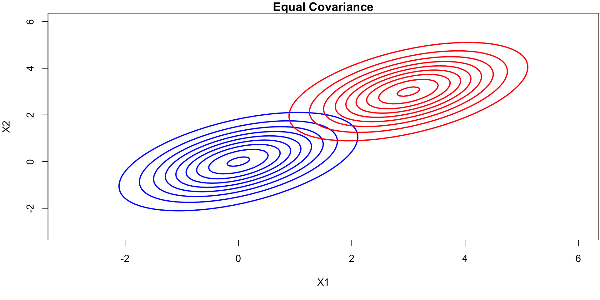
• In the case of \(p > 1\) predictors, the LDA classifier assumes that the observations in the \(k\)th class are drawn from a multivariate Gaussian distribution \(\mathcal{N}(\boldsymbol\mu_k, \boldsymbol\Sigma)\), where \(\boldsymbol\mu_k\) is a class-specific mean vector, and \(\boldsymbol\Sigma\) is a covariance matrix that is common to all \(K\) classes.

• Algebra reveals that the Bayes classifier assigns an observation \(X = x\) to the class for which \[\begin{equation} \delta_k(x) = x^T \boldsymbol\Sigma^{-1} \boldsymbol\mu_k - \frac{1}{2} \boldsymbol\mu_k^T \boldsymbol\Sigma^{-1} \boldsymbol\mu_k + \log(\pi_k) \end{equation}\]

this is the linear function

What does equal Covariance look like?

Source of image [1]

the contours are the same shape and orientation

Contour Plots (equal covariance)

par(mar=c(5,4,1.1,0.1))


# Define the means and shared covariance matrix for the two classes
mean1 <- c(0, 0)
mean2 <- c(3, 3)
cov_matrix <- matrix(c(1, 0.5, 0.5, 1), ncol=2)  # Same covariance matrix for both classes

# Create a grid of points
x <- seq(-3, 6, length=100)
y <- seq(-3, 6, length=100)
grid <- expand.grid(X1 = x, X2 = y)

# Calculate the multivariate normal densities for each class
z1 <- apply(grid, 1, function(x) dmvnorm(x, mean=mean1, sigma=cov_matrix))
z2 <- apply(grid, 1, function(x) dmvnorm(x, mean=mean2, sigma=cov_matrix))

# Reshape for contour plotting
z1_matrix <- matrix(z1, nrow=length(x), ncol=length(y))
z2_matrix <- matrix(z2, nrow=length(x), ncol=length(y))

# Plot the contour plots for the two classes
contour(x, y, z1_matrix, drawlabels=FALSE, col="blue", lwd=2, main="Equal Covariance", xlab="X1", ylab="X2")
contour(x, y, z2_matrix, drawlabels=FALSE, col="red", lwd=2, add=TRUE)

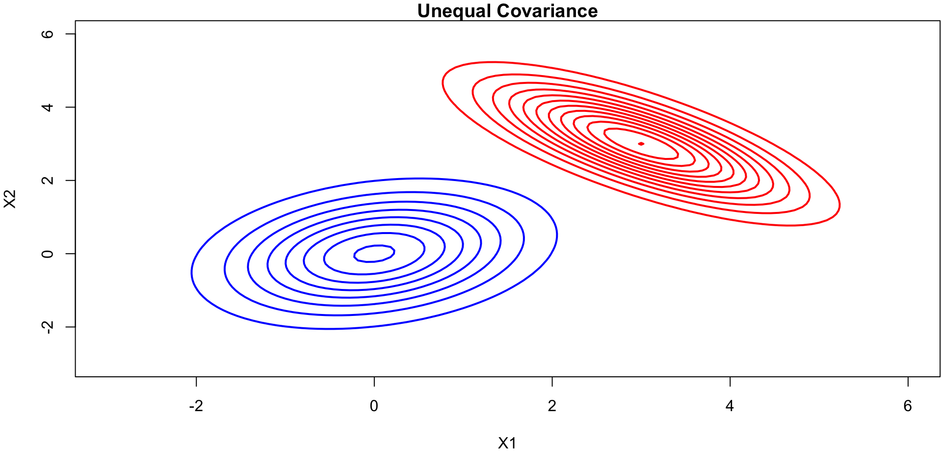
Contour Plots (unequal covariance)

# Load necessary libraries
library(mvtnorm)

par(mar=c(5,4,1.1,0.1))

# Define the means and covariance matrices for the two classes
mean1 <- c(0, 0)
cov1 <- matrix(c(1, 0.25, 0.25, 1), ncol=2)

mean2 <- c(3, 3)
cov2 <- matrix(c(1, -0.75, -0.75, 1), ncol=2)

# Create a grid of points
x <- seq(-3, 6, length=100)
y <- seq(-3, 6, length=100)
grid <- expand.grid(X1 = x, X2 = y)

# Calculate the multivariate normal densities for each class
z1 <- apply(grid, 1, function(x) dmvnorm(x, mean=mean1, sigma=cov1))
z2 <- apply(grid, 1, function(x) dmvnorm(x, mean=mean2, sigma=cov2))

# Reshape for contour plotting
z1_matrix <- matrix(z1, nrow=length(x), ncol=length(y))
z2_matrix <- matrix(z2, nrow=length(x), ncol=length(y))

# Plot the contour plots for the two classes
contour(x, y, z1_matrix, drawlabels=FALSE, col="blue", lwd=2, main="Unequal Covariance", xlab="X1", ylab="X2")
contour(x, y, z2_matrix, drawlabels=FALSE, col="red", lwd=2, add=TRUE)

LDA QDA in 2D

## | cache: true

# Load necessary libraries
library(MASS)

par(mar=c(5,4,1.1,0.1))


# Define the means and shared covariance matrix for the two classes
mean1 <- c(0, 0)
mean2 <- c(3, 3)
cov_matrix <- matrix(c(1, 0.5, 0.5, 1), ncol=2)  # Same covariance matrix for both classes

# Create a grid of points
x <- seq(-3, 6, length=100)
y <- seq(-3, 6, length=100)
grid <- expand.grid(X1 = x, X2 = y)

# Calculate the multivariate normal densities for each class
z1 <- apply(grid, 1, function(x) dmvnorm(x, mean=mean1, sigma=cov_matrix))
z2 <- apply(grid, 1, function(x) dmvnorm(x, mean=mean2, sigma=cov_matrix))

# Reshape for contour plotting
z1_matrix <- matrix(z1, nrow=length(x), ncol=length(y))
z2_matrix <- matrix(z2, nrow=length(x), ncol=length(y))

# Plot the contour plots for the two classes
contour(x, y, z1_matrix, drawlabels=FALSE, col="blue", lwd=2, main="LDA Decision Boundary", xlab="X1", ylab="X2")
contour(x, y, z2_matrix, drawlabels=FALSE, col="red", lwd=2, add=TRUE)

# Plot the LDA decision boundary (it will be linear)
contour(x, y, z1_matrix - z2_matrix, levels=0, drawlabels=FALSE, col="green", lwd=2, lty=2, add=TRUE)

# Add a title and labels
title(main="LDA Decision Boundary")

##| cache: true
 
# Load necessary libraries
library(mvtnorm)

par(mar=c(5,4,1.1,0.1))

# Define the means and covariance matrices for the two classes
mean1 <- c(0, 0)
cov1 <- matrix(c(1, 0.5, 0.5, 1), ncol=2)

mean2 <- c(3, 3)
cov2 <- matrix(c(1, -0.5, -0.5, 1), ncol=2)

# Create a grid of points
x <- seq(-3, 6, length=100)
y <- seq(-3, 6, length=100)
grid <- expand.grid(X1 = x, X2 = y)

# Calculate the multivariate normal densities for each class
z1 <- apply(grid, 1, function(x) dmvnorm(x, mean=mean1, sigma=cov1))
z2 <- apply(grid, 1, function(x) dmvnorm(x, mean=mean2, sigma=cov2))

# Reshape for contour plotting
z1_matrix <- matrix(z1, nrow=length(x), ncol=length(y))
z2_matrix <- matrix(z2, nrow=length(x), ncol=length(y))

# Plot the contour plots for the two classes
contour(x, y, z1_matrix, drawlabels=FALSE, col="blue", lwd=2, main="QDA Decision Boundary", xlab="X1", ylab="X2")
contour(x, y, z2_matrix, drawlabels=FALSE, col="red", lwd=2, add=TRUE)

# Plot the QDA decision boundary where the two densities are equal
contour(x, y, z1_matrix - z2_matrix, levels=0, drawlabels=FALSE, col="green", lwd=2, lty=2, add=TRUE)

Illustration \(p = 2\) and \(K=3\)

ILSR Fig 4.6: Here \(\pi_1 = \pi_2 = \pi_3\) Left: Ellipses that contain 95 % of the probability for each of the three classes are shown. The dashed lines are the Bayes decision boundaries. Right: 20 observations were generated from each class, and the corresponding LDA decision boundaries are indicated using solid black lines. The Bayes decision boundaries are shown as dashed lines.

• equal pis imply same number of training set values

• devision boundardies corresponds to where the contours intersect

• if the bayes decision boundaries were know, they would yeild the fewest mislassification errors, amoung all possilbe classifers

LDA to QDA

• When \(f_k(x)\) are Gaussian densities, with the same covariance matrix \(\boldsymbol\Sigma\) in each class, this leads to linear discriminant analysis.

• With Gaussians but different \(\boldsymbol \Sigma_k\) in each class, we get quadratic discriminant analysis.

• Because the \(\boldsymbol\Sigma_k\) are different, we don’t loose the quadratic terms so we get discriminant function is now

\[\begin{equation} \delta_k(x) = -\frac{1}{2}(x - \mu_k)^T \boldsymbol \Sigma_k^{-1} (x - \mu_k) + \log \pi_k - \frac{1}{2} \log |\Sigma_k| \end{equation}\]

• By altering the forms for (f_k(x)), we get different classifiers.

where \(|\Sigma_k|\) is the determinant of the covariance matrix

QDA Parameter Estimates

For QDA/LDA the parameters estimates are given by: \[ \begin{align} \hat{\mu}_k &= \frac{1}{n_k} \sum_{i : y_i = k} x_i, & \hat{\pi}_k &= \frac{n_k}{n} \end{align} \]

For QDA the estimate for covariance is: \[\hat{\Sigma}_k = \frac{1}{n_k - 1} \sum_{i : y_i = k} (x_i - \mu_k)(x_i - \mu_k)^\top,\]

LDA Parameter Estimates

For QDA/LDA the parameters estimates are given by: \[ \begin{align} \hat{\mu}_k &= \frac{1}{n_k} \sum_{i : y_i = k} x_i, & \hat{\pi}_k &= \frac{n_k}{n} \end{align} \]

For LDA, one uses the pooled covariance estimator:

\[\hat{\Sigma} = \frac{1}{n - K} \sum_{k=1}^{K} \sum_{i : y_i = k} (x_i - \mu_k)(x_i - \mu_k)^\top.\]

Summary

Both LDA and QDA assumes each class follows an underlying Gaussian distribution

LDA

• assumes equal variance across classes

• PRO: easier to fit

• CON: less flexible

QDA

• doesn’t assume equal variance across classes

• PRO: often leads to a lower error rate

• CON: needs more data

Bias-variance tradeoff: the LDA can be too simple whereas the QDA has a higher risk of overfitting to our data.

Example: Iris

4 variables 3 species 50 samples/class:

• Setosa (blue)
• Versicolor (green)
• Virginica (orange)

par(mar = c(3.9, 3.9, 0, 1))        # reduce even more 
lookup <- c(setosa='blue', versicola='green', virginica='orange')
col.ind <- lookup[iris$Species]
pairs(iris[-5], pch=21, col="gray", bg=col.ind)

LDA fitted model

Let’s fit the LDA classifier using all 4 predictors

lda.fit <- lda(Species ~ ., data = iris)
lda.fit

...
Prior probabilities of groups:
    setosa versicolor  virginica 
 0.3333333  0.3333333  0.3333333 

Group means:
           Sepal.Length Sepal.Width Petal.Length Petal.Width
setosa            5.006       3.428        1.462       0.246
versicolor        5.936       2.770        4.260       1.326
virginica         6.588       2.974        5.552       2.026

...

• The output shows that the prior probabilities of each group (setosa, versicolor, and virginica) are all equal at 0.33.
• The group means section shows the mean values of each input variable (sepal length, sepal width, petal length, and petal width) for each group.

coefficients of linear discriminants: are the weights of the linear combination of the input variables that best separates the groups. - The “LD1” and “LD2” columns represent the first and second linear discriminant functions, respectively. - Each row represents the weight of a particular input variable in the linear combination.

the proportion of trace is the proportion of the total variability in the input variables that is explained by each linear discriminant function. - the first linear discriminant function (LD1) explains 99.12% of the total variability, - the second linear discriminant function (LD2) explains only 0.88%. This indicates that most of the discriminatory power of the input variables is captured by the first linear discriminant function.

Plotted fit

plot(Sepal.Width ~ Sepal.Length, data = iris, pch=21, col="gray", bg= col.ind)
points(lda.fit$means[,1], lda.fit$means[,2], pch=21, cex=2,
       col="black", bg=lookup)

Classification Table

LDA classifies all but 3 of the 150 training samples correctly.

lda.pred <- predict(lda.fit) # this is a list
names(lda.pred)

[1] "class"     "posterior" "x"        

table(iris$Species, lda.pred$class)

            
             setosa versicolor virginica
  setosa         50          0         0
  versicolor      0         48         2
  virginica       0          1        49

This of course is the training error so it may be overly optimistic.

Posterior Probabilties

We can obtain the posterior probabilities if we so desire:

round(lda.pred$posterior, 3)

    setosa versicolor virginica
1        1      0.000     0.000
2        1      0.000     0.000
3        1      0.000     0.000
4        1      0.000     0.000
5        1      0.000     0.000
6        1      0.000     0.000
7        1      0.000     0.000
8        1      0.000     0.000
9        1      0.000     0.000
10       1      0.000     0.000
11       1      0.000     0.000
12       1      0.000     0.000
13       1      0.000     0.000
14       1      0.000     0.000
15       1      0.000     0.000
16       1      0.000     0.000
17       1      0.000     0.000
18       1      0.000     0.000
19       1      0.000     0.000
20       1      0.000     0.000
21       1      0.000     0.000
22       1      0.000     0.000
23       1      0.000     0.000
24       1      0.000     0.000
25       1      0.000     0.000
26       1      0.000     0.000
27       1      0.000     0.000
28       1      0.000     0.000
29       1      0.000     0.000
30       1      0.000     0.000
31       1      0.000     0.000
32       1      0.000     0.000
33       1      0.000     0.000
34       1      0.000     0.000
35       1      0.000     0.000
36       1      0.000     0.000
37       1      0.000     0.000
38       1      0.000     0.000
39       1      0.000     0.000
40       1      0.000     0.000
41       1      0.000     0.000
42       1      0.000     0.000
43       1      0.000     0.000
44       1      0.000     0.000
45       1      0.000     0.000
46       1      0.000     0.000
47       1      0.000     0.000
48       1      0.000     0.000
49       1      0.000     0.000
50       1      0.000     0.000
51       0      1.000     0.000
52       0      0.999     0.001
53       0      0.996     0.004
54       0      1.000     0.000
55       0      0.996     0.004
56       0      0.999     0.001
57       0      0.986     0.014
58       0      1.000     0.000
59       0      1.000     0.000
60       0      1.000     0.000
61       0      1.000     0.000
62       0      0.999     0.001
63       0      1.000     0.000
64       0      0.994     0.006
65       0      1.000     0.000
66       0      1.000     0.000
67       0      0.981     0.019
68       0      1.000     0.000
69       0      0.960     0.040
70       0      1.000     0.000
71       0      0.253     0.747
72       0      1.000     0.000
73       0      0.816     0.184
74       0      1.000     0.000
75       0      1.000     0.000
76       0      1.000     0.000
77       0      0.998     0.002
78       0      0.689     0.311
79       0      0.993     0.007
80       0      1.000     0.000
81       0      1.000     0.000
82       0      1.000     0.000
83       0      1.000     0.000
84       0      0.143     0.857
85       0      0.964     0.036
86       0      0.994     0.006
87       0      0.998     0.002
88       0      0.999     0.001
89       0      1.000     0.000
90       0      1.000     0.000
91       0      0.999     0.001
92       0      0.998     0.002
93       0      1.000     0.000
94       0      1.000     0.000
95       0      1.000     0.000
96       0      1.000     0.000
97       0      1.000     0.000
98       0      1.000     0.000
99       0      1.000     0.000
100      0      1.000     0.000
101      0      0.000     1.000
102      0      0.001     0.999
103      0      0.000     1.000
104      0      0.001     0.999
105      0      0.000     1.000
106      0      0.000     1.000
107      0      0.049     0.951
108      0      0.000     1.000
109      0      0.000     1.000
110      0      0.000     1.000
111      0      0.013     0.987
112      0      0.002     0.998
113      0      0.000     1.000
114      0      0.000     1.000
115      0      0.000     1.000
116      0      0.000     1.000
117      0      0.006     0.994
118      0      0.000     1.000
119      0      0.000     1.000
120      0      0.221     0.779
121      0      0.000     1.000
122      0      0.001     0.999
123      0      0.000     1.000
124      0      0.097     0.903
125      0      0.000     1.000
126      0      0.003     0.997
127      0      0.188     0.812
128      0      0.134     0.866
129      0      0.000     1.000
130      0      0.104     0.896
131      0      0.000     1.000
132      0      0.001     0.999
133      0      0.000     1.000
134      0      0.729     0.271
135      0      0.066     0.934
136      0      0.000     1.000
137      0      0.000     1.000
138      0      0.006     0.994
139      0      0.193     0.807
140      0      0.001     0.999
141      0      0.000     1.000
142      0      0.000     1.000
143      0      0.001     0.999
144      0      0.000     1.000
145      0      0.000     1.000
146      0      0.000     1.000
147      0      0.006     0.994
148      0      0.003     0.997
149      0      0.000     1.000
150      0      0.018     0.982

Fitting QDA

We would similarly fit QDA to the iris data using the qda() function.

To help visualize this, let’s use two predictors Sepal.Length and Sepal.Width:

# Fit LDA and QDA models
lda.fit <- lda(Species ~ Sepal.Length + Sepal.Width, data = iris)
qda.fit <- qda(Species ~ Sepal.Length + Sepal.Width, data = iris)

Visualization

iClicker

iClicker

Which of the following is an advantage of QDA over LDA?

1. It is simpler to implement than LDA

2. It performs better when the covariance matrices of the classes are equal

3. It is more flexible and can handle non-linear decision boundaries

4. It requires fewer data points to estimate parameters

Correct answer: C.

Assumptions

LDA assumes the data is:

1. LDA makes no assumptions on the data

2. Gaussian with different covariance for each class

3. Gaussian with equal covariance for all classes

4. Gaussian with equal means for call classes

Correct answer: C.