Data 311: Machine Learning

Lecture 6: Logistic Regression

Dr. Irene Vrbik

University of British Columbia Okanagan

Introduction

• Lately we’ve been focused on the regression problem–that is, the supervised machine learning problem when our response variable is a continuous quantity.

• Machine learning algorithms that aim at predicting a categorical (AKA qualitative) response are referred to as classification techniques.

• In this section, rather than trying to predict a continuous responses, we will be trying to classify observations in to categories (AKA classes)

as with the regression setting, we’ll start off simple.

These is a very simple technique (although KNN is even simplier)

we often first predict the probabilities

These the posts are the only ones that made sense to me:

• https://online.stat.psu.edu/stat504/lesson/6/6.1

• https://statisticaloddsandends.wordpress.com/2019/10/31/understanding-the-components-of-a-generalized-linear-model-glm/

Misnomer: it has regression in the name but it’s actually a model for classification

Outline

• Generalized Linear Model

• Link and Inverse Link Function

• Logistic Regression

• Interpretation of Coefficients

• Generalized Linear Model (glm)

• Metrics for Classification

• Bayes Classifier

Text Definition

Logistic Regression is a supervised statistical method used for binary¹ classification problems.

• Examples: Spam detection, medical diagnosis, …

Note that the name is a bit of a misnomer; this is not a method for regression (predicting a continuous \(y\)), this is a classification technique (predicting categorical \(y\))

The method was named by the statistician David Cox in 1958.

1. can be extended to more than two classes but this works ideally with two classes

Mathematical Definition

As we will see, logistic regression outputs a probability like:

\[ p(Y=1 \mid X) = \frac{e^{\beta_0 + \beta_1 X_1 \dots + \beta_p X_p}}{1 + e^{\beta_0 + \beta_1 X_1 + \dots + \beta_p X_p}} \]

Under the hood we are modelling: \[ \text{log odds} = \beta_0 + \beta_1 X_1 \dots + \beta_p X_p \]

models the conditional probability an observation belonging to a certain class given \(X\).

instead of modeling \(y\) directly, we model the log-odds as a linear function of the predictor variables.

log odds = the logarithm of the odds of the probability of success to the probability of failure

odds = ratio of the P(event occuring)/P(event not occuring)

odds of rolling a 4 on a die is 1:5 (1/6 \(\div\) 5/6)

This linearity in the log-odds makes logistic regression similar to linear regression, thus justifying the term “regression.”

Although the target variable in logistic regression is categorical, the underlying mechanics of the model (like minimizing a loss function and using predictors to estimate coefficients) are similar to linear regression models.

Why not Linear Regression?

Consider coding categories as numeric, say we had recorded eye colour:

\[ Y = \begin{cases} 1 & \text{Green}\\ 2 & \text{Blue} \\ 3 & \text{Brown} \end{cases} \]

Suppose we fed this into a linear model.

Question: What would a prediction of 1.5 signify?

• Mid-way beween green and blue is brown?

• but avg between blue and green would be brown?

• any number smaller than 1 is green

• any number >3 is brown?

• 1.5-2.5 is blue. But the answer would change if we coded them a different number

• can’t treat numeric codings as numeric values

• think carfeully about how we set it up

• diffent colour 50-50 chance between green and brown.

• what would a 50/50 change been green and blue look like?

Class levels

• Numeric codings for a response fed into a continuous model assumes a natural order, or hierarchy.

• For multi-class categorical data, this is simply inappropriate.

• But what about a binary classification problem?

\[ Y = \begin{cases} 1 & \text{Green}\\ 0 & \text{Not green} \\ \end{cases} \]

Can we use this in a linear model such that a predicted value of 0.5 suggests a 50-50 chance that a person’s eye colour is green?

Promising? treat predicted ys as probablities

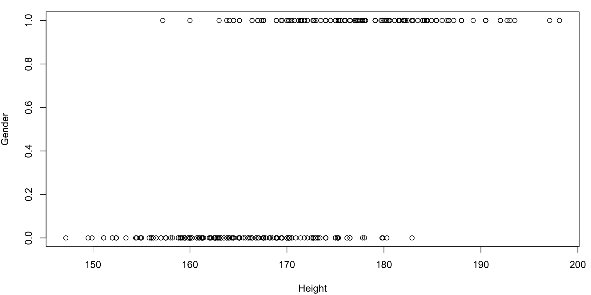
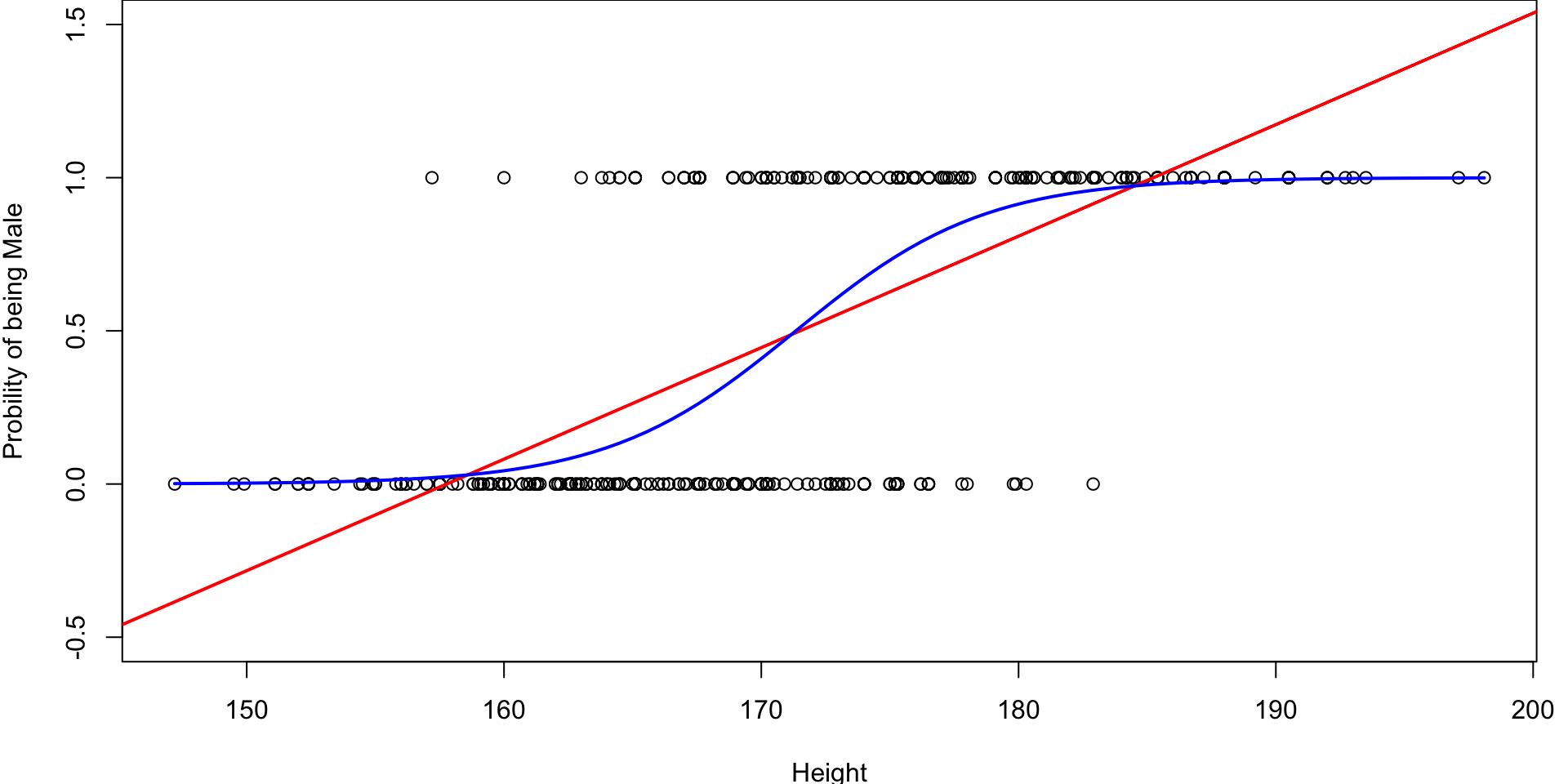
Example: body

• Consider the body (from the gclus package) data set from previous lectures

• Let’s attempt to model the recorded Gender as a linear function of Height.

# install.packages(gclus) # DONT ever include in Rmd/Rscript
library(gclus)            # cannot data() before library() 
data(body); attach(body)  # cannot attach() before data()
fit1 <- lm(Gender~Height) # cannot call Gender/Height before attach()
plot(Gender~Height)       # note the formula option Y~X

A scatterplot of Gender on the y-axis and Height on the X axis. Points fall along two horizontal lines: where Gender = 1 (indicating males) and Gender =0 (indicating females).

Example: body

Multiple Linear Regression

Recall the linear regression model: \[\begin{equation} Y = \beta_0 + \beta_1 X_1 + \cdots + \beta_p X_p + \epsilon \end{equation}\]

• \(Y\) is the random, quantitative response variable
• \(X_j\) is the \(j^{th}\) random predictor variable
• \(\beta_0\) is the intercept
• \(\beta_j\) from \(j = 1, \dots p\) are the regression coefficients
• \(\epsilon\) is the error term

Two basic assumptions of this model are the additivity in the parameters, and the normally distributed errors https://bookdown.org/pingapang9/linear_models_bookdown/logistic.html

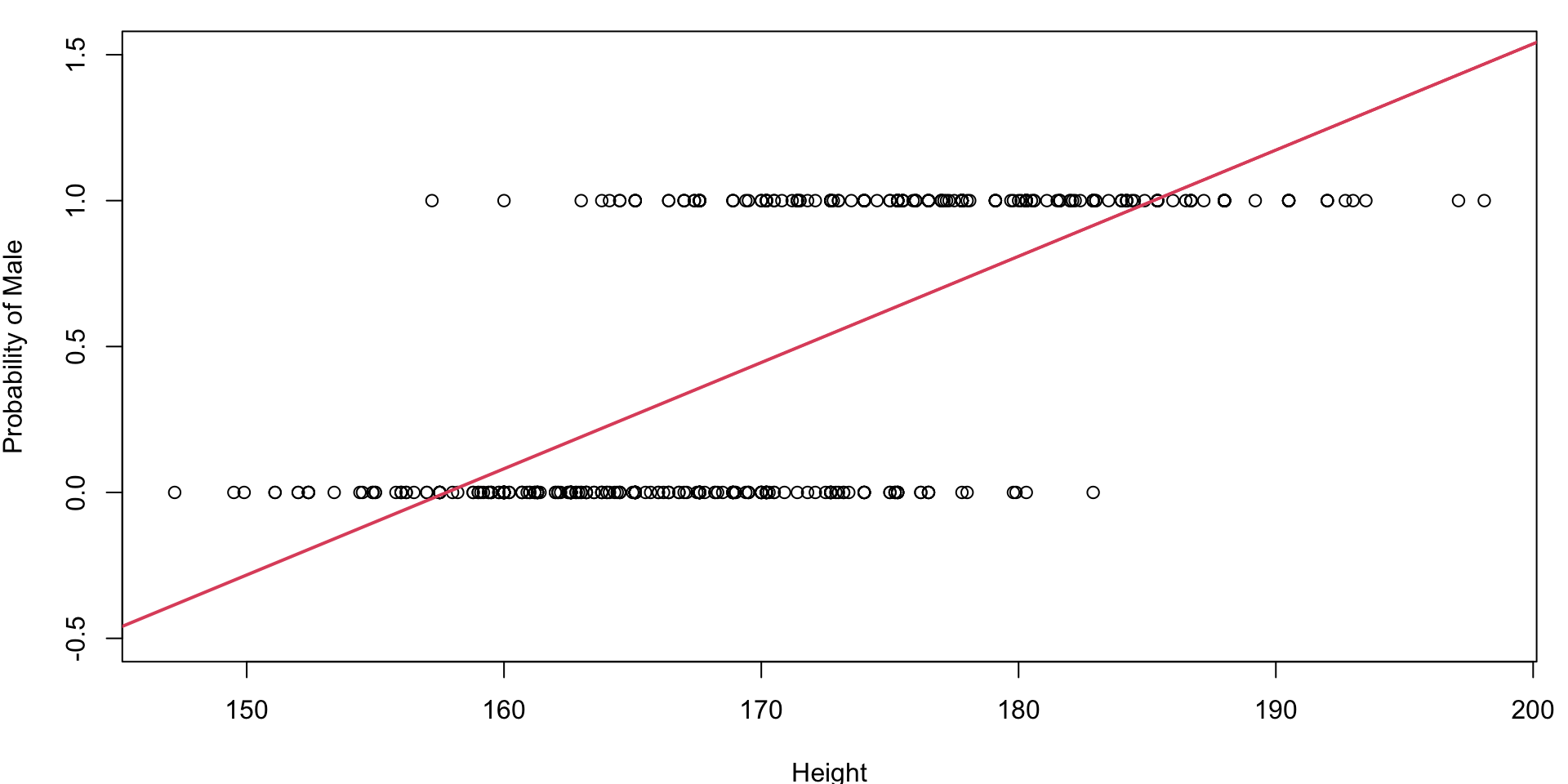
Fitted line

plot(Gender~Height, ylab = "Probability of Male")
abline(fit1, lwd=2, col=2)

Question: What’s wrong with this?

(see next slide for hint)

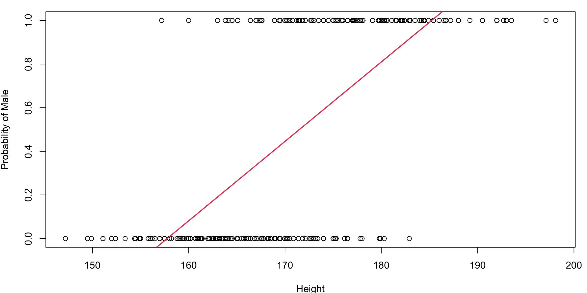
Same Plot (zoomed out)

plot(Gender~Height, ylim=c(-0.5, 1.5), ylab="Probability of Male")
abline(fit1, lwd=2, col=2)

• get predictions >1 and <0 (negative probabilities)

• cap it at 1?

Generalized Linear Model

Rather than modeling continuous \(Y \in (-\infty, \infty)\) using: \[\begin{equation} Y = \underbrace{\beta_0 + \beta_1 X_1 + \cdots + \beta_p X_p}_{\eta} \end{equation}\]

A GLM consists of three components:

1. Systematic component: a linear combination of the predictors (\(\eta\))
2. Random component: the probability distribution of \(Y\)
3. Link function: Connects \(E[Y]\) to \(\eta\).

The systematic component (aka linear predictor \(\eta\)) a linear combination of the predictor variable.

The systematic component specifies the probability distribution of the response variable (dependent variable). Specifies the pdf of \(y\)

Link function denoted by \(g\) relates linear predictor (η) to the expected value of the response variable. Connects the mean of the pdf to \(\eta\)

Systematic Component

• The systematic component represents the linear combination of the independent variables.

• It is typically expressed as \[\begin{equation} \eta = \beta_0 + \beta_1 X_1 + \dots \beta_p X_p \end{equation}\] where

• \(\eta\) is the linear predictor,

• \(\beta_0, \beta_1, \dots \beta_p\) are the coefficients. , and

• \(X_1, X_2, \dots, X_p\) are the predictors.

• A GLM is a flexible and powerful framework for modeling the relationship between a dependent variable and one or more independent variables.
• It generalizes the classical linear regression model by allowing for different types of response variables, including non-continuous data, and by using a link function to connect the linear predictor to the response variable. G so we need a function to map \(- \infty < y < \infty\) to value from 0 to 1

The coefficients are interpreted as the change in the log-odds of the outcome for a one-unit change in the predictor variable, similar to how coefficients are interpreted in linear regression but on a different scale.

Random Component

• We assume that \(y_1, \dots, y_n\) are samples of independent random variables \(Y_1, \dots, Y_n\) respectively.

• The random component specifies the probability distribution \(f(y_i; \theta_i)\) of the response variable.

• For GLM’s the probability distributions are assumed to arise from the Exponential family.

• Logistic regression is a type of GLM where the response variable is binary.

exponential family is a parametric set of probability distributions of a certain form, specified below.

Exponential family

• The exponential family includes a large class of probability distributions e.g. normal, binomial, Poisson and gamma distributions, among others.

Classical regression assumes:

• \(Y_i \sim \text{Normal}(\mu_i, \sigma^2)\)
• \(E[Y_i] = \mu_i\)

Logistic regression assumes

• \(Y_i \sim \text{Bernoulli}(\pi_i)\)
• \(E[Y_i] = \pi_i\)

Link and Inverse Link Function

The mean of the distribution, \(\mu = {E}[Y_i]\) depends on the independent variables, \(X\), through the link function

\[\begin{align*} \eta &= g(\mu) \end{align*}\]

\[\begin{align*} g^{-1}(\eta) &= \mu \end{align*}\]

The inverse link function (aka activation function), \(g^{−1}\), transforms the linear predictor \(\eta = \beta_0 + \beta_1 X_1 + \dots \beta_p X_p\) back to the scale of the response variable.

Link function

The link function is a transformation that relates the mean of the response variable to the linear predictor.

\[\begin{equation} \eta = g(\mu) \end{equation}\]

where \(\mu = {E}[Y_i]\)

Link function Linear Regression

The link function is a transformation that relates the mean of the response variable to the linear predictor.

\[\begin{equation} \eta = g(\mu) \end{equation}\]

In classical linear regression, we use the identity link:

\[\begin{align} \eta &= 1(\mu) \\ \beta_0 + \beta_1 X_1 + \dots \beta_p X_p&= \mu \phantom{\beta_0 + \beta_1 x_1 } \end{align}\]

where \(\mu = E[Y_i]\) where \(Y_i \sim N(\mu_i, \sigma^2)\)

just multiply by 1

Logit Link

In logistic regression, we use the logit link, i.e.

\[\begin{align} \eta = g(\mu) = \text{logit}(\mu) &= \ln \left( \frac{\mu}{1-\mu} \right) \\ \beta_0 + \beta_1 X_1 + \dots \beta_p X_p &= \ln \left( \frac{\pi_i}{1-\pi_i} \right)\\ \end{align}\]

where \(\mu = E[Y_i] = \pi_i = P(Y_i = 1)\) when \(Y_i \sim \text{Bernoulli}(\pi_i)\)

The logit function maps the probability of the dependent variable being 1 to a linear combination of independent variables.

then we can write:

\[\eta = g(\pi_i) = \ln \left( \frac{\pi_i}{1-\pi_i} \right)\]

log-odds = \(\eta\)

• Odds are traditionally used instead of probabilities in horse-racing, since they relate more naturally to the correct betting strategy

• odds take on values from 0 (very small probs) to positive infinity (when prob = 1)

• log-odds will go from -infty to infty

• log-odds may feel weird but they have a nice interpretation

Logit Function

More generally if \(p\) is a probability, then

• \(\dfrac{p}{1 − p}\) is the corresponding odds and

• logit \(p\) = \(\ln \left( \dfrac{p}{1-p}\right)\) is the logit of the probability \(p\)

• this value is sometimes referred to as the log-odds or “logits”

Since the logit is the natural logarithm of odds it is sometimes referred to as the log-odds.

• odds take on values from 0 (very small probs) to positive infinity (when prob = 1)

• log-odds will go from -infty to infty

• log-odds may feel weird but they have a nice interpretation

Plotted log-odds

Probabilities converted to the logit (log-odds) scale. Notice how the logit functions allows us to map values from 0 to 1 to values from negative infinity to infinty.

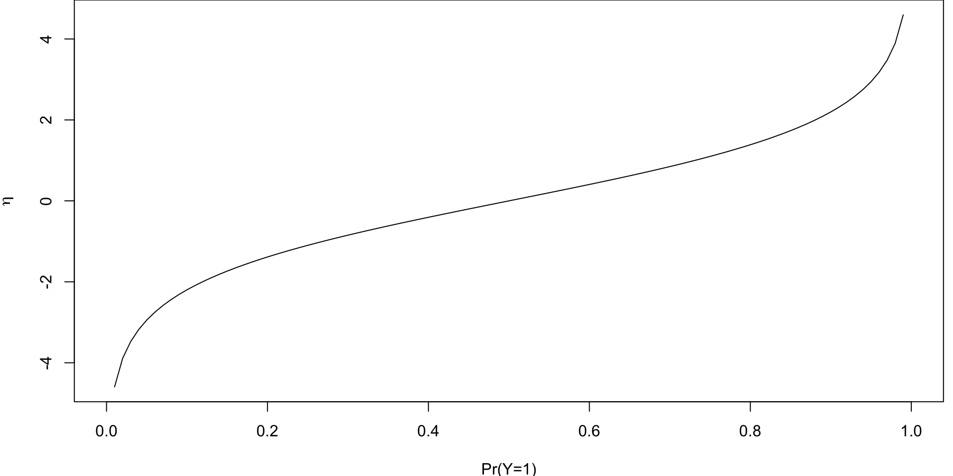
If \(p = 0.5 \implies\) the odds \(\left(\frac{p}{1-p}\right)\) are even and the log-odds is zero.

Negative (resp. positive) logits represent probabilities below (resp. above) one half.

log-odds = \(\eta\)

logit maps \(\Pr(Y=1)\) to \(eta\)

logisitic maps \(eta\) to \(\Pr(Y=1)\)

• “A curve representing log-odds on the y-axis and probability on the x-axis. The curve approaches negative infinity for very small probabilities (close to 0) and infinity for very large probabilities (close to 1). The curve is a smooth s-shaped rotated by 90 degrees and mirrored.

Logistic Function

\[\begin{align} \text{logit } (\pi_i) &= \eta\\ \pi_i &= \text{logit}^{-1}(\eta) \end{align}\]

\[\begin{align} \text{Recall: } g(\mu) &= \eta\\ \mu &= g^{-1}(\eta) \end{align}\]

The inverse of the logit function, i.e. the activation/inverse link function \(g^{-1}\), is the standard logisitic function¹

\[\begin{align} \pi_i = \text{Sigmoid}(\eta) &= \dfrac{1}{1 + e^{-\eta}} = \dfrac{1}{1+ e^{-(\beta_0 + \beta_1 X_1 + \cdots \beta_p X_p)}} \end{align}\]

An inverse function is a function that reverses the effect of the original function.

• If \(f\) maps an x to y, then its inverse function \(f^{-1}\) maps y back to x.

Let’s remind ourselves what \(\pi_i\) is… it’s the \(Pr(Y_i) = 1\) in a bernoulli trial. …

Also let’s simplify the fraction.

\[\begin{align} P(Y_i = 1 \mid X) &= \dfrac{e^{(\beta_0 + \beta_1 X_1 + \cdots \beta_p X_p)}}{e^{(\beta_0 + \beta_1 X_1 + \cdots \beta_p X_p)}+ 1} \end{align}\]

“standard” implies with the supremum of the values of the function = 1, the logistic growth rate = 1, and function’s midpoint = 0.

1. also known as the sigmoid function.

Plotted Logistic Function

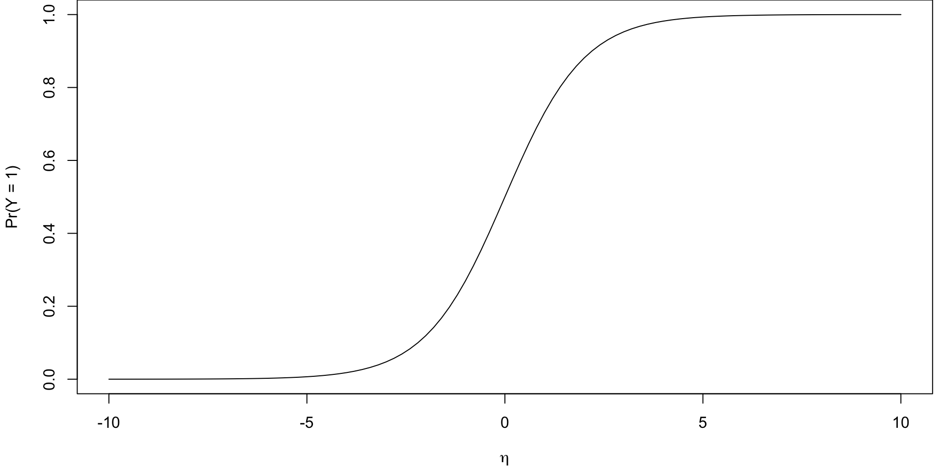
It is a S-shaped curve (sigmoid curve) that allows us to go back from logits to probabilities.

curve representing probabilities on the y-axis and log-odds on the x-axis. The curve approaches 0 large as lod-odds becomes more negative and approaches 1 as the log-odds becomes more positive (when log-odds = 0, probablity = 0.5). The curve is a smooth s-shape.

For any value of log-odds i can convert to a number between 0 and 1. The smaller the logodds, the smaller the probabilitily

From Line to S-curve

Instead of trying to fit a line to this data, let’s try to fit something more like this S-curve so that \(0 \leq \pi_i \leq 1\)

• Fitting a straight line doesn’t make sense so instead we fit an S-curve goes from 0 to 1

• so our predictions will fall on this blue sigmoid curve and correspond to the \(P(Y=1 \mid X)\)

  • so gives the probabilty of male given height

• We need a function that will transform any point on the red line to a point on this blue S-curve

Logistic Regression

Link Function \[ \begin{align} g(\mu) &= \eta\\ \text{log odds} = \ln\left(\frac{\mu}{1-\mu}\right) &= \beta_0 + \beta_1 X_1 + \dots + \beta_p X_p \end{align} \]

Inverse Link Function

\[ \begin{align} g^{-1}( \eta) &= \dfrac{e^{\sum_{j=1}^p\beta_j X_j}}{1+ e^{\sum_{i=1}^p\beta_i X_i}} = \dfrac{1}{1+e^{-\sum_{j=1}^p\beta_j X_j}} = \Pr(Y = 1)\\ \end{align} \]

\[ \begin{align} g(\mu) &= \eta \\ \ln \left( \frac{\mu}{1-\mu}\right) &= \beta_0 + \beta_1 X_1 + \dots \beta_p X_p\\ g^{-1}( \eta) &= \dfrac{e^{\sum_{j=1}^p\beta_j X_j}}{1+ e^{\sum_{i=1}^p\beta_i X_i}} = \dfrac{1}{1+e^{-\sum_{j=1}^p\beta_j X_j}}\\ \end{align} \]

where \(g(\cdot)\) is the Logit Function and \(g^{-1}(\cdot)\) is the Logistic Function.

Assumptions of Logistic Regression

• Binary dependent variable: The response variable \(Y\) must be binary (i.e., it takes on only two possible outcomes, such as 0 and 1, yes or no, success or failure).
• Independence of observations¹
• Linearity of the Logit: There should be a linear relationship between the logit of the outcome (log-odds) and each continuous predictor variable.

• No multicollinearity.

\(Y_i \sim \text{Bernoulli}(\pi_i)\) and \(\mu = E[Y_i] = \pi_i\)

1. Violations of this assumption often occur in time-series data or clustered data.

iClicker

logit function

In the context of logistic regression, what does the logit function represent?

1. The probability of success in a binary outcome.
2. The natural logarithm of the odds of success.
3. The inverse of the probability of failure.
4. The square root of the expected value of the response variable.

Correct answer: B

It represents the log-odds that \(Y = 1\).

Note that we can easily convert back to probabilities

\[ p = \frac{e^{\beta_0 + \beta_1 x_1 + \beta_2 x_2 + \ldots + \beta_p x_p}}{1 + e^{\beta_0 + \beta_1 x_1 + \beta_2 x_2 + \ldots + \beta_p x_p}} \]

iClicker

logit function

In a logistic regression model, what is the range of values that \(Y\) can take?

1. Any real number
2. Any integer
3. 0 or 1
4. 0 to infinity

Correct answer: C

Interpretation of Coefficients

Since probability \(\pi_i\) is non-linear as \(X\) varies¹, we cannot interpret the coefficients as we did in regular regression.

The best we can do is talk about the direction:

• Holding all other variables constant, if \(\beta_j\) is positive, then an increase in \(X_j\) is associated with an increase in \(\pi_i\)

• Holding all other variables constant, if \(\beta_j\) is negative, then an increase in \(X_j\) is associated with a decrease in \(\pi_i\).

Difference: in the linear regression we were modeling \(y\) in logistic regression we are modeling the log-odds \[ \text{log odds} = \ln\left( \frac{\pi_i}{1 - \pi_i}\right) = \beta_0 + \beta_1X_1 + \dots \beta_p X_p \]

• In logistic regression model, increasing X by one unit changes the log odds by β1 (4.4).

• Equivalently, it multiplies the odds by \(e^{\beta_1}\)

• it’ll matter where we are in terms of X (see example)

1. in logistic regression, increasing \(X\) by one unit changes the log odds by \(\beta_1\)

Estimation

Let \(G_1\) be the set of observations where \(Y=1\), let \(G_0\) be the set of observations where \(Y=0\), and let \(\boldsymbol{\beta}\) be the set of coefficients. The likelihood is given by:

\[ l(\boldsymbol{\beta}) = \prod_{i \in G_1 }P(y_i=1\mid x_i)^{y_i}\prod_{h \in G_0 }(1-P(y_i=1\mid x_h))^{1-y_i} \]

To fit the parameters of these models, we use maximum likelihood ¹ estimation.

Not through least squares anymore (we don’t have a concept of a residual anymore)

• beta = vector of beta

• likelihood of betas = product of probabilities given the predictors

• one of the most common ways we fit models

• the MLE estimates are the most likely values of the betas given the data we saw

• try to find the best fitting squiggle s

we can’t use OLS since log(0)

find the \(\beta\)s that maximize this likelihood

1. Maximum likelihood is a core concept of statistical inference, but is outside the scope of this course (see STAT 401, and some others, instead)

From lm() to glm()

You can fit a logistic regression using the glm() function.

glm(formula, family = gaussian, data, ...)

Arguments	Description
formula	a symbolic description of the model to be fitted, eg Y~ X1 + X2
family	a description of the error distribution and link function to be used in the model ?family
data	data frame (usually your training set)

Click things to go to the help file!

glm families

• To perform logistic regression with a binary outcome we need to set family = "binomial"¹.

• Other options (not be covered in this course) include:

  • family = "gaussian" same as lm()

  • family = "poisson" for predicting counts

  • family = multinomial for \(>2\) classes

  • family = binomial('probit') probit regression (a common alternative to logistic regression)

• poisson for modelling count data
• multinomial for modeling >2 levels in a categorical variable
• logit is not the only function we can use to map the linear predictor to a probability (common alternative is probit - inverse CDF of a normal distribution)
• In practice, both probit and logistic regression can yield similar results for many datasets, and the choice between them often depends on the specific problem, theoretical considerations, and the preference of the researcher.

Descriptions of families: https://www.youtube.com/watch?v=DDP62EUMRFs&ab_channel=KasperWelbers

glm are very flexible and powerful

1. Think binomial distribution (can be either “success” or “failure”)

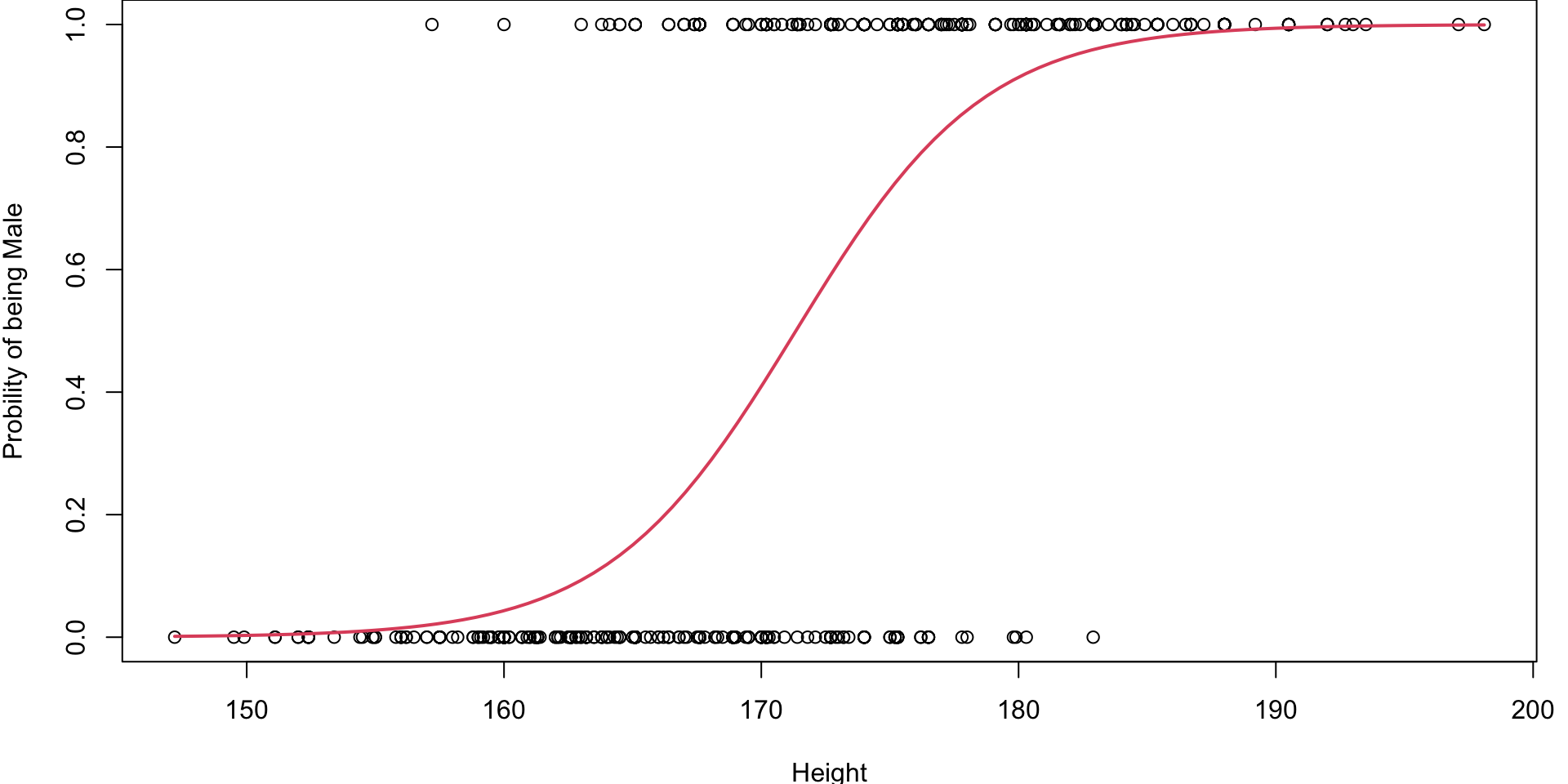
Fitted Logistics Regression Plot

We are using the Logistic Function with the fitted \(\hat \beta\) values to plot the fitted S-curve

# Fit the logistic regression model
simlog <- glm(factor(Gender) ~ Height , family="binomial")

# store the beta hats for easy referencing
betas <- coef(simlog)  

# plot the data (renaming the y-axis)
plot(Gender~Height, ylab="Probility of being Male")

# plot the fitted curve p(x) = e^(b0+b2x)/(1 + e^(b0+b2x))
curve(
  (exp(betas[1] + betas[2]*x))/(1+exp(betas[1] + betas[2]*x)),
  add=TRUE, # superimposes onto scatterplot (otherwise new plot)
  lwd=2, # line width (make the line a bit thicker)
  col=2) # 2 = red  

This will be the “best” S curve in terms of the maximum likelihood function.

All probabilities lie between 0 and 1 when log-reg is used

to convert the linear combo of betas to probabilities we have to use the inverse logit, aka the logistic function

• i’m using curve() but you can plot the predict()ed values for a lengthy sequence of plausible x values

Fitted Logistics Regression Plot

Summary Output

summary(simlog)

...
Coefficients:
             Estimate Std. Error z value Pr(>|z|)    
(Intercept) -46.76328    4.00571  -11.67   <2e-16 ***
Height        0.27292    0.02339   11.67   <2e-16 ***
---
Signif. codes:  0 '***' 0.001 '**' 0.01 '*' 0.05 '.' 0.1 ' ' 1

(Dispersion parameter for binomial family taken to be 1)

    Null deviance: 702.52  on 506  degrees of freedom
Residual deviance: 389.59  on 505  degrees of freedom
AIC: 393.59

Number of Fisher Scoring iterations: 5
...

We can use this output to assess what predictors are useful in classifying samples - the p value corresponds to the Wald test (but similar interpretation to the t-test from regression) to test if it’s statistically significant

interpretation of coefs:

• \(\beta_0\) when height = 0 the log-odds of being a male is -46.76 (nonsensical)

• \(\beta_1\) For every one cm increase in height, you would expect the log-odd of male to increase by 0.2792

• notice how we don’t have an R-2 cuz we don’t have residuals We’ll to compare log reg models in a different way than we did for normal regression

iClicker

Interpretation of coefficients

In a logistic regression model, the coefficient \(\beta_1\) associated with a predictor variable \(X_1\)​ is interpreted as:

1. The change in the predicted probability of the outcome for a one-unit increase in \(X_1\)​, holding all other variables constant.
2. The change in the odds of the outcome for a one-unit increase in \(X_1\), holding all other variables constant.
3. The change in the log-odds of the outcome for a one-unit increase in \(X_1\), holding all other variables constant.
4. The change in the outcome value for a one-unit increase in \(X_1\)​, holding all other variables constant.

Correct answer: C

iClicker

Parameter estimation

Which method is used to estimate the coefficients (parameters) in a logistic regression model?

1. Ordinary Least Squares (OLS)
2. Maximum Likelihood Estimation (MLE)
3. Method of Moments
4. Bayesian Estimation

Correct answer: B

Multiple Logistic Regression

As with linear regression we could just as easily add predictors.

# Fit the logistic regression model
mult_log_reg <- glm(factor(Gender) ~ Height + WaistG + BicepG, family="binomial")
summary(mult_log_reg)

...
Coefficients:
             Estimate Std. Error z value Pr(>|z|)    
(Intercept) -55.32670    5.51960 -10.024  < 2e-16 ***
Height        0.21534    0.02864   7.520 5.50e-14 ***
WaistG        0.05167    0.02891   1.787   0.0739 .  
BicepG        0.46541    0.08265   5.631 1.79e-08 ***
---
Signif. codes:  0 '***' 0.001 '**' 0.01 '*' 0.05 '.' 0.1 ' ' 1

(Dispersion parameter for binomial family taken to be 1)

    Null deviance: 702.52  on 506  degrees of freedom
Residual deviance: 232.90  on 503  degrees of freedom
AIC: 240.9

Number of Fisher Scoring iterations: 6
...

we could also include interaction terms

Recall Gender = 1 (male) Gender = 0 (female)

So we are modeling the log-odds of an individual being a male

. Deviance and Model Fit:

• Null Deviance = 702.52: This is the deviance of a model with no predictors (only an intercept). It serves as a baseline.

• Residual Deviance = 232.90: This is the deviance of the model with the predictors Height, WaistG, and BicepG included. A large reduction from the null deviance suggests that the model with predictors fits the data better.

• Degrees of Freedom: The null deviance has 506 degrees of freedom (number of observations minus 1), and the residual deviance has 503 degrees of freedom (506 observations minus 3 predictors minus 1 intercept).

• AIC = 240.9: The Akaike Information Criterion (AIC) measures the goodness of fit while penalizing for the number of parameters. Lower AIC values indicate a better model fit.

Model fit

You will notice that we no longer have a \(R^2\) or adjusted R-square value as we did in the linear regression case.

• the concept of “variance explained” doesn’t not apply.
• furthermore, since the observed y values are 0 and 1, transforming those values to the linear form using log(p/1-p) will produce -\(\infty\) and \(\infty\) so there are no ways to calculate residuals

• Deviance is a lack of fit measure (the smaller the better) that plays the role of RSS for a broader class of models.
• Null Deviance is the deviance of a model with no predictors (only an intercept). It serves as a baseline.
• The residual deviance measures the deviance that remains unexplained after fitting the logistic regression model.

• Instead of sum of squares, logistic regression uses deviance
• other metrics exist (example psuedo R^2 value)
• The residual deviance tells us how well the response variable can be predicted by a model with p predictor variables.
• The lower the value, the better the model is able to predict the value of the response variable.

we will see deviance come up again later in the course

• The Akaike Information Criterion (AIC) is a goodness of fit measure that penalizing for the number of parameters.

• AIC (the smaller the better)
• model comparison When comparing two or more logistic regression models, you can use the likelihood ratio test (e.g. anova(mod1, mod2, test = Chisq)), which involves comparing the residual deviance of the models.

The deviance is a function of the log-likelihood

Metrics for Classification

We can evaluate the model by making predictions on new unseen data and assessing its performance; see Lecture 3

• error/misclassification rate
• accuracy
• precision
• recall
• specificity
• F1-score

These can all be computed from a so-called classification table (aka confusion matrix)

unlike the AIC and deviance that evaluates the goodness of fit to the training data these evaluation metrics will evaluate accuracy of these models on unseen data (similar concept to MSE train and MSE test.

• Also the ROC curve Receiver Operating Characteristic (ROC) curves graphically represent the trade-off between true positive rate (recall) and false positive rate (1-specificity) for different classification thresholds.

• The Area Under the ROC Curve (AUC-ROC) measures the model’s ability to discriminate between classes. A higher AUC-ROC indicates better discrimination.

we will look at these metrics in more detail next lecture

Validation of Predicted Values

With a fitted logistic regression model the predict() function (see ?predict.glm) we can either predict the categorical response or output a probability.

predict(mod_fit, newdata=testing) # outputs the log-odds
predict(mod_fit, newdata=testing, type="response") # outputs probabilities

or more generally for glm models

note that you can eitehr output in terms of probabilities or classification vectors

From Probability to Classification

• Logistic Regression produces a probabilistic classifier¹.

  \[ \begin{cases} 1 & \text{ if } \Pr(Y=1 \mid x) \geq 0.5\\ 0 & \text{ otherwise} \end{cases} \]

• Since we are considering only binary outpus, \(P(Y=1 \mid x)=0.5\) defines a decision boundary.

For predicting classification we consider

\[ \max \{ P(Y=0 \mid x), P(Y=1 \mid x) \} \]

We can obtain these probabilities in R using the predict() function on the fitted model (see lab)

Where is this boundary for the body example in terms of \(X\)?

• Although, logistic regression, outs a probability it’s usually used for classification

• For example if the probability of male is greater than 50% then we’ll classify it as obese

Like KNN classification we say, whichever class has the highest prob gets assigned that obs (Bayes classifier)

1. a ML model or algorithm designed to categorize input data into one or more discrete classes or categories

Plot of Probability Boundary

Highlight the observations that would be misclassified by this classifier

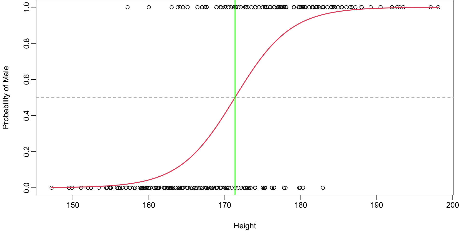
Height boundary

\[ \log \left(\frac{0.5}{0.5-0}\right) = {\hat\beta_0 + \hat\beta_1 X} \]

\[ \begin{align} \implies && \log \left(1\right) &= {\hat\beta_0 + \hat\beta_1 X} \\ \implies && X &= -\frac{\hat\beta_0}{\hat\beta_1} \end{align} \]

recall log(1) = 0 \[ 0.5 =\dfrac{e^{\beta_0 + \beta_1 X}}{1+ e^{\hat\beta_0 + \hat\beta_1 X}} \]

If Height \(> -\dfrac{ -46.76}{0.27} = 171.34\) we would predict Male.

This defines a very simple classifier in terms of \(x\) = Height

Classification Table

For classification, we often summarize performance in a classification table (aka confusion matrix).

tab <- table(Gender, predict(simlog, type="response")>0.5)
rownames(tab) <- c("1 - male", "0 - female")
colnames(tab) <- c("predicted male", "predicted female")
kable(tab)

Note

Typically the off-diagonals are errors and diagonal are correctly classified observations

In this case, the off-diagonals are errors (and diagonal are correctly classified obs.).

Classification Table

	predicted male	predicted female
1 - male	216	44
0 - female	45	202

Table 1: This table presents the confusion matrix which summarizes the performance of a classification model in predicting Gender. It shows the counts of correctly and incorrectly classified instances for both males and females. The rows represent the actual gender, while the columns represent the predicted gender.

Confusion Matrix

	predicted male	predicted female
1 - male	216	44
0 - female	45	202

• True Positives (TP): Correctly predicted males (216)

• False Positives (FP): Females incorrectly predicted as males (45)

• True Negatives (TN): Correctly predicted females (202)

• False Negatives (FN): Males incorrectly predicted as females (44)

Error Rate

In words, the error rate (aka misclassification rate) calculates the proportion of misclassifications that are made by \(\hat f\):

\[\begin{align} \frac{1}{n} \sum_{i=1}^n I(y_i \neq \hat y_i) = \frac{\text{total misclassified}}{\text{total no. observations}} \end{align}\]

and \(\hat y_i\) is the predicted class label for the \(i\)th observation \(x_i\) using \(\hat f\) and \[\begin{equation} I(y_i \neq \hat y_i)= \begin{cases} 1, y_i \neq \hat y_i\\ 0, \text{otherwise} \end{cases} \end{equation}\]

The error rate for this classification table is \[\begin{align} \dfrac{44+45}{216+44+45+202} = \dfrac{89}{507} = 0.1755424 \approx 17.6% \end{align}\]

no r squared values! (theres about 10 ways people have thought about doing this)

There are other way to access predicted classifications later

Problems

• the regular diagnostics plots don’t really apply for this model

• multiple categories? (back to the reference label)

• we can extend this model (but there are better options )

• next lecture will be more mathy

Accuracy

\[ \text{Accuracy} = \frac{TP + TN}{TP + TN + FP + FN} \]

\[\begin{align} &=\frac{TP + TN}{n} = \frac{216 + 202}{507} = \frac{418}{507} \\ &= \frac{\text{correct predictions}}{\text{total predictions}} = 0.8244576 \end{align}\]

Accuracy is calculated as the proportion of correctly classified instances out of all instances.

Precision

\[\begin{align} \text{Precision} &= \frac{TP}{TP + FP}\\ &=\frac{216}{216 + 45} = \frac{216}{261} \\ &= 0.8275862 \end{align}\]

Precision (also known as Positive Predictive Value) is the proportion of true positives among all predicted positives.

Recall

Recall (Sensitivity or True Positive Rate)

\[\begin{align} \text{Recall} &= \frac{TP}{TP + FN}\\ &=\frac{216}{216 + 44} = \frac{216}{260} \\ &= 0.8275862 \end{align}\]

Recall (also known as Sensitivity or True Positive Rate) is the proportion of true positives among all actual positives.

Specificity (TN rate)

	Pred male	Pred female
Actual male	216	44
Actual female	45	202

\[\begin{align} \text{Specificity} &= \frac{TN}{TN + FP} \\ &= \frac{202}{202 + 45} = \frac{202}{247} = 0.8178138 \\ &= \frac{\text{true negatives}}{\text{actual negatives}} \end{align}\]

Specificity (True Negative Rate) is the proportion of true negatives among all actual negatives.

F1-score

\[ \begin{align} \text{F1} &= \dfrac{2 \times \text{Precision} \times \text{Recall}} {\text{Precision} + \text{Recall}}\\ &= \dfrac{2 \times 0.8275862 \times 0.8307692} {0.8275862+ 0.8307692}\\ &= 0.8291747 \end{align} \]

Note

F1-score is particularly useful when there is an uneven class distribution (i.e. “unbalanced” classes).

The F1-Score is the harmonic mean of precision and recall, providing a single measure that balances both.

Summary of Metrics

• Accuracy: 82.45%

• Precision: 82.76%

• Recall: 83.08%

• Specificity: 81.78%

• F1-Score: 82.92%

• Accuracy measures overall correctness.

• Precision measures the accuracy of the positive predictions.

• Recall measures how well the model identifies true positives.

• Specificity measures how well the model identifies true negatives.

• F1-Score balances precision and recall

Tackles the weakness of precision. Use specificity when avoiding false positives among actual negatives is the priority.

• e.g. quality control or screenings for rare conditions where false positives could lead to unnecessary further actions.
• Focus: Specificity measures the ability to correctly identify all actual negatives, minimizing false positives.
• When to Use: Specificity is important when it is crucial to correctly identify negatives, avoiding false positives, such as in quality control or screenings for rare conditions where false positives could lead to unnecessary further actions.
• Strength: Good at avoiding false positives among actual negatives.
• Weakness: Does not account for false negatives, so it may fail to identify many positives if it focuses too much on being specific to negatives.

Key Distinction:

• Precision minimizes false positives among the predicted positives.

• Specificity minimizes false positives among the actual negatives.

Summary:

• Use precision when avoiding false positives in positive predictions is crucial.

• Use recall when avoiding false negatives and capturing all positives is critical.

• Use specificity when avoiding false positives among actual negatives is the priority.

Which metric to use?

• Accuracy: When the dataset is balanced (i.e., both classes are equally represented)
• Precision: use when the cost of false positives is high, e.g. spam
• Recall: use when the cost of false negatives is high, e.g. disease screening
• Specificity: use when its important to correctly identify negative cases, e.g. fraud detection
• F1-score: When there is an imbalance¹ between precision and recall, and you want a single metric that accounts for both. Useful in imbalanced datasets.

SPAM why Not Recall?: High recall would mean catching all spam emails, but at the risk of also catching too many legitimate emails.

disease why not precision

• Accuracy can misleading in the presence of class imbalance.
  • For example, if 95% of emails are not spam, a model that always predicts “not spam” will have 95% accuracy but is useless for detecting spam.
• High precision may come at the cost of low recall, meaning the model may miss many actual positive cases. -

1. aka “unbalanced classes”

Testing vs Training error rate

• Akin to our earlier discussions with MSE for regression, we are generally interested with the error rate from the testing set rather than the training set.

• That is, for a set of new observations \((x_0, y_0)\), a good classifier achieves the smallest test error on average: \[\begin{equation} E[I(y_0 \neq \hat y_0))], \end{equation}\] where \(\hat y_0\) is the predicted class label for \(x_0\) that uses \(\hat f\).

Comments

• Is it reasonable to assume a linear relationship between the log-odds and the predictors?

Your guess is as good as mine…(no more residuals to check)

• assuming a linear relationship between log odds and predictors (log odds actually get mapped to -infty and infty so we don’t have the concept of a residual so we can’t do the diagnostics.

• predict Y = 1 Probabilty 1 goes to infinicty, Y = 0 goes to negative infinity

• What if we have multiple categories for our response?

No problem, bit of a change in notation and mathematics, but R can handle it just fine. family = "multinomial"

✏️ Next class we’ll move on to another (more natural) model for classification (Bring some paper and a pen!)

• unstable parameters when the separation between two classes is large (next class of models we consider do not suffer from this problem)

• DA is a more naturally extensions into the multivariate case