Data 311: Machine Learning

Lecture 5: Regression Models Part 2

Dr. Irene Vrbik

University of British Columbia Okanagan

Outline

We are in the supervised machine learning setting, we will investigate:

1. Interaction (linear regression model)
2. Categorical Predictors (linear regression model)
3. Interaction with Mixed Predictors (linear regression model)
4. Polynomial Regression
5. KNN Regression (non-parametric approach)

• “interact” related to the marketing term synergy, in regression Interaction)
• we are trying to predict an outcome, or dependent variable, in relation to changes in the predictors, or independent variables, for a population by determining a linear relationship between the combination of all the independent variables and the dependent variable of a sample from that population.

READ ME

Include something about the AIC for model selection?

Example: Clock Auction

• The data give the selling price, Price at auction of 32 antique grandfather clocks.

• Also recorded is the age of the clock (Age) and the number of people who made a bid (Bidders).

• This data can be downloadable here

Note: this data is tab delimited; values within the dataset are separated by tab characters. One way to read this into R is to use read.delim().

What is the natural \(Y\) output for this data?

• Price

Clock Auction Data

(dat <- read.delim("data/clockauction", sep="\t"))

First 6 lines of 32

3D Scatter plot

library(plotly)
fig <- plot_ly(dat, x = ~Age, y = ~Bidders, z = ~Price)
fig <- fig %>% add_markers()
fig

Correlation

correlation matrix (see ?cor)

cor(dat)

               Age    Bidders     Price
Age      1.0000000 -0.2537491 0.7302332
Bidders -0.2537491  1.0000000 0.3946404
Price    0.7302332  0.3946404 1.0000000

It is reassuring that Price seems to be linearly related to the Age and Bidders. Notice that Age and Bidders have a slight negative correlation.

recall correlation ranges from -1 to 1 and larger in magnitude values indicate a stronger linear relationship.

Pairwise scatterplot

Another way that you could investigate correlation is through a pairwise scatterplot, obtained using plot()

# reduce the margins surrounding the plots
par(mar = c(1, 1, 0.1, 1))      
attach(dat)
plot(dat)

• as age increases, it is more of an antique which drives the price up

• as the number of bidders increases, the price tends to go up

• there doesn’t seem to be much of a relationship at all between age and bidders

SLR with Age

agelm <- lm(Price~Age)
summary(agelm) 

...
Call:
lm(formula = Price ~ Age)

Coefficients:
            Estimate Std. Error t value Pr(>|t|)    
(Intercept)  -191.66     263.89  -0.726    0.473    
Age            10.48       1.79   5.854  2.1e-06 ***
---
Signif. codes:  0 '***' 0.001 '**' 0.01 '*' 0.05 '.' 0.1 ' ' 1

Residual standard error: 273 on 30 degrees of freedom
Multiple R-squared:  0.5332,    Adjusted R-squared:  0.5177 
F-statistic: 34.27 on 1 and 30 DF,  p-value: 2.096e-06
...

• look at the solo effect of age on price, this does seem to be a significant predictor (very small p-value) strong evidence of a linear relationship between age and price

• multiple r squared of 0.5332 so we can explain roughly 53 percent of the variation in price using just age in a linear model

• the coef is positive so for each increase of one year in age i expect the price to go up by 10.4790949 on average

some lines of output were supressed to conserve space

SLR with Bidders

bidlm <- lm(Price~Bidders)
summary(bidlm)

...
Call:
lm(formula = Price ~ Bidders)

Coefficients:
            Estimate Std. Error t value Pr(>|t|)   
(Intercept)   806.40     230.68   3.496  0.00149 **
Bidders        54.64      23.23   2.352  0.02540 * 
---
Signif. codes:  0 '***' 0.001 '**' 0.01 '*' 0.05 '.' 0.1 ' ' 1

Residual standard error: 367.2 on 30 degrees of freedom
Multiple R-squared:  0.1557,    Adjusted R-squared:  0.1276 
F-statistic: 5.534 on 1 and 30 DF,  p-value: 0.0254
...

• Bidders have a sig p-value

• for each addition person bidding no the clock, we expect the price to go up by 54.6362045 on average.

• compared with age, bidders is not as good as age (smaller r-squared value)

• only explains about 16 of the variation in Price can be determined by Age.

iClicker

iClicker: SLR comparison

Which model explains a higher percentage of the variance in Price?

1. SLR with Age

2. SLR with Bidders

3. Both models explain the same percentage

4. None of the models explain any variance

Correct answer: A. This model has a righer \(R^2\) and smaller RSE

MLR without Interaction

ablm <- lm(Price~Age+Bidders); summary(ablm)

...
Call:
lm(formula = Price ~ Age + Bidders)

Coefficients:
              Estimate Std. Error t value Pr(>|t|)    
(Intercept) -1336.7221   173.3561  -7.711 1.67e-08 ***
Age            12.7362     0.9024  14.114 1.60e-14 ***
Bidders        85.8151     8.7058   9.857 9.14e-11 ***
---
Signif. codes:  0 '***' 0.001 '**' 0.01 '*' 0.05 '.' 0.1 ' ' 1

Residual standard error: 133.1 on 29 degrees of freedom
Multiple R-squared:  0.8927,    Adjusted R-squared:  0.8853 
F-statistic: 120.7 on 2 and 29 DF,  p-value: 8.769e-15
...

• AKA Full First Order MLR (significant F value)

• large improvement in r-squared. including both Bidders and Age in the Model has allowed us to explain more of the variability in Price as compared to SLRM for Bidders and Age individually.

  • age explaines around 53% of the variation

  • bidders explaines around 16% of the variation

  • 89% of the variance (> 16+53 = 69)

• none of these calculates work in a vacum, beta_j is the change in y expected when the remaining variables are held at the same value or are fixed.

• it allows you to assess the affect of each varialbe in issolation from the others

iClicker

Fitted MLR model

What is the fitted model?

1. Price = Age \(\times\) 12.74 + Bidders \(\times\) 85.82

2. Price = -1336.72 + Age \(\times\) 12.74 + Bidders \(\times\) 85.82

3. Price = -1336.72 + 12.74 + 85.82

4. Price = -1336.72 \(\times \beta_0\) + Age \(\times\) 12.74 + Bidders \(\times\) 85.82

Correct answer: B

Interpretation of Coefficients

• \(\beta_1\): For a clock with a given amount of Bidders, an increase of 1 year in the age of the clock is associated with a $12.74 increase in the mean price of the clock.

• \(\beta_2\) : For a clock with given age, an increase of 1 Bidder is associated with a $85.82 increase in the mean selling price.

Important

Notice that the specific value of age (resp. bidders) does not affect the interpretation of \(\beta_1\) (resp. \(\beta_2\))

Notice that for any fixed number of bidders, a one unit increase in Age will results in a 85.82 increase in Price on average.

Setting Bidders values

Fitted model:

Price = -1336.72 + Age \(\times\) 12.74 + Bidders \(\times\) 85.82

Example 1: when we have 6 bidders Price is calculated:

= -1336.72 + Age \(\times\) 12.74 + 6 \(\times\) 85.82

= -821.8 + Age \(\times\) 12.74

Example 2: when we have 12 bidders Price is calculated:

= -1336.72 + Age \(\times\) 12.74 + 12 \(\times\) 85.82

= -306.88 + Age \(\times\) 12.74

Notice how both lines have the same slope

• slope is the same
• intercept is different

MLR Visualization (no interaction)

with 2 qualitative predictors

library(RColorBrewer)
cf.mod <- coef(ablm)
par(mar = sm.mar)
plot(Price~Age, ylim = c(100, 3000))
ivec <- seq(from = min(Bidders), to = max(Bidders))
icol <- brewer.pal(n = length(ivec), name = "Spectral")
for (i in 1:length(ivec)){
  abline(a = cf.mod[1] + cf.mod["Bidders"]*ivec[i], b = cf.mod["Age"], col = icol[i])
}
points(Age, Price)
legend("topleft", legend = ivec, col = icol, ncol = 3, lty = 1, title = "Number of Bidders")

A scatter plot with Price on the Y-axis and Age on the X axis. There are 11 parallel lines plotted indicating the fitted line for specified values of bidders (= 5, 6, …, 15).

but maybe there is some synergy between these two variables. In other words, maybe the affect of age on price depends on how many bidders are interested.

x1.seq <- seq(min(Age),max(Age),length.out=25)
x2.seq <- seq(min(Bidders),max(Bidders),length.out=25)
z <- t(outer(x1.seq, x2.seq, function(x,y) cf.mod[1]+cf.mod[2]*x+cf.mod[3]*y))

fig %>% add_surface(x = ~x1.seq, y = ~x2.seq, z = ~z, showscale = FALSE, opacity = 0.5)

A 3D scatterplot of the clock data with the fitted additive MLR model (no interaction) depicted as a plane. This plane is the surface that minimizes the sum of squared residuals

Interaction

Motivation

• Suppose that the affect of Age on Price actually depends on how many Bidders there are.

• Similarly, the affect of Bidders on Price might depend on the Age of the clock.

• We can allow the coefficient of a predictor to vary based on the value(s) of the other predictor(s) by including an additional interaction term¹

Synergy effect refers to a situation where the combined effect of multiple variables on the response variable is greater (or sometimes different) than the sum of their individual effects.

For instance, the affect of one more bidder on a relatively recent clock won’t be as strong as the affect of one extra bidder on a really old clock.

in other words, the interaction between variables can produce an outcome that is not simply the additive effect of each variable acting independently.

1. In marketing, this interaction term is refereed to as a synergy effect

Interaction Model

With 2 predictors

\[\begin{equation} Y = \beta_0 + \beta_1 X_{1} + \beta_2 X_{2} + \beta_3 X_{1} X_{2} + \epsilon \end{equation}\]

• \(Y\) is the response variable
• \(X_{j}\) is the \(j^{th}\) predictor variable
• \(\beta_0\) is the intercept (unknown)
• \(\beta_j\) are the regression coefficients (unknown)
• \(\epsilon\) is the error, assumed \(\epsilon \sim N(0, \sigma^2)\).

In marketing, this is known as a synergy effect, and in statistics it is referred to as an interaction effect

• same assumptions on the error term

• interpretation of betajs get a bit more hairy

• i’ve dropped the subscript i for ease of viewing

MLR with Interaction

\[\begin{align} Y &= \beta_0 + \beta_1 X_1+ \beta_2 X_2+ \beta_3 X_1 X_2 \end{align}\]

\[\begin{align} \phantom{Y} &= \beta_0 + \beta_2 X_2 + (\beta_1 + \beta_3 X_2) X_1 \end{align}\]

\[\begin{align} \phantom{Y} &= \tilde{\beta_0} + \tilde{\beta_1} X_1 \phantom{+ (\beta_1 + \beta_3 X_2) X_1 } \end{align}\]

where \(\tilde\beta_1 = (\beta_1 + \beta_3 X_2)\) and \(\tilde\beta_0 = (\beta_0 + \beta_2 X_2)\). We can view this as a “new” coefficient for \(X_1\), denoted \(\tilde{\beta_1}\), which is a function of \(X_2\) so that the association between \(X_1\) and \(Y\) is no longer constant, but depends on the value \(x_2\)

• The interaction term can be thought of as a new predictor variable that we created by multiplying age and bidders together.

• It too, will have a regression coefficient associated with it that requires estimate

A similar argument can be made for a new \(\tilde{\beta_2}\) associated with \(X_2\)

Interaction in R

# same as lm(Price~ Age + Bidders + Age*Bidders) 
ilm <- lm(Price ~ Age*Bidders); summary(ilm)

...
Coefficients:
            Estimate Std. Error t value Pr(>|t|)    
(Intercept) 322.7544   293.3251   1.100  0.28056    
Age           0.8733     2.0197   0.432  0.66877    
Bidders     -93.4099    29.7077  -3.144  0.00392 ** 
Age:Bidders   1.2979     0.2110   6.150 1.22e-06 ***

Residual standard error: 88.37 on 28 degrees of freedom
Multiple R-squared:  0.9544,    Adjusted R-squared:  0.9495 
F-statistic: 195.2 on 3 and 28 DF,  p-value: < 2.2e-16
...

What do you notice in this output?

• Age does not have a significant p-value (we’ll come back to that)

• Bidders has a large negative value. Does bidders have a negative effect on price? (no way!)

• \(R^2\) go up to 95%. but we should really be looking at the adjusted R-squared which takes into account that more predictors are always going to do better

Hierarchical Pricinciple

You will notice that the so-called main effect of the Age predictor does not have a significant \(p\)-value; resist the temptation to remove it from the model!

Hierarchical principal

If the interaction effect is significant you should also keep the main effects even if they have non-significant p-values

Interpretation gets really tricky otherwise

This is done to maintain the interpretability of the model and ensure that the interaction term is correctly interpreted.

Interpretation of Coefficients

Theoretical Model

Price = \(\beta_0\) + \(\beta_1\cdot\)(Age) + \(\beta_2\cdot\)(Bidders) + \(\beta_3\cdot\)(Age \(\cdot\) Bidders)

Fitted Model

Price = \(\hat\beta_0\) + \(\hat\beta_1\cdot\)(Age) + \(\hat\beta_2\cdot\)(Bidders) + \(\hat\beta_3\cdot\)(Age \(\cdot\) Bidders)

\(\phantom{\texttt{Price}}\) = 322.8 + 0.9 (Age) -93.4 (Bidders) + 1.3(Age \(\cdot\) Bidders)

• \(\beta_1\) is the effect of Age when Bidders = 0.
• Since a clock needs to have at least 1 bidder to be sold \(\beta_1\) is meaningless by itself.

So how can we communicate the affect of Age on Price?

• Like the intercept of the simple linear regression model the interpretation of \(\beta_1\) can be nonsensical (there is no auction price if there are no bidders)
• HOW? that answer will depend on how many Bidders there are.
• Better: the effect of Age is 0.9 + 1.3 \(\cdot\) Bidders

Fitted Model with 6 bidders

\[\begin{align} &\texttt{Price} = \hat\beta_0 + \hat\beta_1\texttt{Age} + \hat\beta_2\cdot\texttt{Bidders} + \hat\beta_3\cdot\texttt{Age} \cdot \texttt{Bidders}\\ &= 322.75 + 0.87\cdot\texttt{Age} -93.41\cdot\texttt{Bidders} + 1.3\cdot\texttt{Age} \cdot \texttt{Bidders}\\ &= 322.75 + ( 0.87 + 1.3\cdot \texttt{Bidders})\texttt{Age} -93.41\cdot\texttt{Bidders} \end{align}\]

Notice now the multiplier associated with Age now depends on the value of Bidders.

For example, if Bidders = 6, Price is given:

\[\begin{align} &= 322.75 + (0.87 + 1.3\cdot 6)\texttt{Age} -93.41 (6) \\ &= 322.75 + (8.66)\texttt{Age} -560.46 \\ &= -237.71 + (8.66)\texttt{Age} \end{align}\]

When there are 6 bidders we expect the price of the clock to increase in auction sale by 8.66 for every 1 year increase in the clock

• note the -93.41 coefficient doesn’t not cause lead to a drop in price, but gets absorbed in this case to a lower intercept

• with a 110 year old clock, we can estimated price of 714.89

Fitted Model with 12 bidders

\[\begin{align} &\texttt{Price} = \hat\beta_0 + \hat\beta_1\texttt{Age} + \hat\beta_2\cdot\texttt{Bidders} + \hat\beta_3\cdot\texttt{Age} \cdot \texttt{Bidders}\\ &= 322.75 + 0.87\cdot\texttt{Age} -93.41\cdot\texttt{Bidders} + 1.3\cdot\texttt{Age} \cdot \texttt{Bidders}\\ &= 322.75 + ( 0.87 + 1.3\cdot \texttt{Bidders})\texttt{Age} -93.41\cdot\texttt{Bidders} \end{align}\]

Notice now the multiplier associated with Age now depends on the value of Bidders.

Eg. Bidders = 12, Price is given:

\[\begin{align} &= 322.75 + (0.87 + 1.3\cdot 12)\texttt{Age} -93.41 (12) \\ &= 322.75 + (16.45)\texttt{Age} -1120.92 \\ &= -798.16 + (16.45)\texttt{Age} \end{align}\]

When there are 12 bidders we expect the price of the clock to increase in auction sale by 16.45 for every additional year on the clocks life

• with a 110 year old clock, we can estimated price of 1023.34

Predicted price of 150-year-old clocks

\[\begin{align} &\texttt{Price} = \hat\beta_0 + \hat\beta_1\texttt{Age} + \hat\beta_2\cdot\texttt{Bidders} + \hat\beta_3\cdot\texttt{Age} \cdot \texttt{Bidders}\\ &= 322.75 + 0.87\cdot\texttt{Age} -93.41\cdot\texttt{Bidders} + 1.3\cdot\texttt{Age} \cdot \texttt{Bidders}\\ &= 322.75 + ( 1.3\texttt{Age} -93.41 ) \texttt{Bidders} + 0.87 \cdot \texttt{Age} \end{align}\]

Notice now the multiplier associated with Bidders now depends on the value of Age.

Eg. Age = 150, Price is given:

\[\begin{align*} &= 322.75 + ( 1.3\cdot 150 -93.41 ) \texttt{Bidders} + 0.87 \cdot 150 \\ &= 322.75 + ( 101.27 ) \cdot \texttt{Bidders} + 130.99 \\ &= 453.75 + ( 101.27 ) \cdot \texttt{Bidders} \end{align*}\]

• with a 7 bidders, we can estimated price of 1162.64

Predicting using R

predict(ilm, newdata = data.frame(Age = 105, Bidders = 6))

      1 
671.666 

predict(ilm, newdata = data.frame(Age = 105, Bidders = 12))

       1 
928.8824 

predict(ilm, newdata = data.frame(Age = 150, Bidders = 7))

       1 
1162.671 

Important

newdata must be a data frame with columns that match the names of your predictors used in the lm() fit. If omitted, the fitted values in your training set will be used. For more information see ?predict.lm

iClicker negative price

What is the main reason these predictions might not be reliable?

predict(ilm, data.frame(Age = 30, Bidders = 7))

        1 
-32.35781 

predict(ilm, data.frame(Age = 125, Bidders = 88))

       1 
6488.723 

1. The assumptions are not being met
2. Age and Bidders should be the same number
3. We are extrapolating outside our observed data range
4. The model is underfitting

Hint: it might be useful to revisit the Pairwise scatterplot

Correct answer: C

• Extrapolating Age range: 108, 194
• Extrapolating Bidders range: 5, 15

cf.mod <- coef(ilm)
x1.seq <- seq(min(Age),max(Age),length.out=25)
x2.seq <- seq(min(Bidders),max(Bidders),length.out=25)
z <- t(outer(x1.seq, x2.seq, function(x,y) cf.mod[1]+cf.mod[2]*x+cf.mod[3]*y+ cf.mod[4]*x*y))

fig %>% add_surface(x = ~x1.seq, y = ~x2.seq, z = ~z, showscale = FALSE    ,
                    surfacecol = "gray", opacity = 0.5)

A 3D scatterplot of the clock data with the fitted MLR model with interaction depicted by a (non-flat) surface.

A 3D scatterplot of the clock data with the fitted MLR with interaction depicted as a curved (non-flat) surface.

Interaction Model with set Bidders

library(RColorBrewer)
par(mar = sm.mar)
plot(Price~Age, ylim = c(100, 3000))
ivec <- seq(from = min(Bidders), to = max(Bidders))
icol <- brewer.pal(n = length(ivec), name = "Spectral")
for (i in 1:length(ivec)){
  abline(a = cf.mod[1] + cf.mod[3]*ivec[i], 
         b = cf.mod[2] + cf.mod[4]*ivec[i], 
         col = icol[i])
}
points(Age, Price)
legend("topleft", legend = ivec, col = icol, ncol = 3, lty = 1, title = "Number of Bidders")

I have set this for the 11 possible values for integer Bidders, but you could imagine how a continuous RV would have a infinite continuum of lines that we can view as the surface in the 3d plot

Categorical Predictors

• So far we’ve assumed that our predictors are continuous valued when we’ve fit a regression.

• But there is no real problem if instead we have categorical (i.e. qualitative) values

• Let’s motivate this through an example.

Example body

This data set contains the following on 507 individuals:

• 21 body dimension measurements (eg. wrist and ankle girth)

• Age, Weight (in kg), Height (in cm), and Gender¹ .

You can find this in the gclus library as body.

library(gclus)
data(body); attach(body)
dim(body)

[1] 507  25

1. Gender was recorded as a binary variable (1 - male, 0 - female).

body data set

Notice that gender is considered an integer here 1 = male, 0 = female

Let’s regress Weight on some of these predictors.

Scatterplot Weight vs Height

slr <- lm(Weight~Height)
par(mar = c(4.9, 3.9, 1, 1))        # reduce white space around figure
plot(Weight~Height)
abline(slr, col =4, lwd = 3)

Scatter plot of Weight versus Height with the fitted Simple Linear Regression model (Weight regressed on Height) superimposed over the data. The scatter plot and fitted line indicate a positive linear relationship

Incorporating Gender

But we know more, eg. gender.

par(mar = c(4.9, 3.9, 0, 0.5))        # reduce even more 
plot(Weight~Height, col=Gender+1)   # 1 = black, 2 = red (3 = green, 4 = blue ...)
abline(slr, col =4, lwd = 2)
legend("topleft", col=c(2,1), pch=1, legend = c("Male", "Female"))

Question: how do we incorporate categorical variables into this model?

Scatter plot of Weight versus Height with the fitted Simple Linear Regression model (Weight regressed on Height) superimposed over the data. Points are coloured according to gender (black = female, red = male). The scatter plot and fitted line indicate a positive linear relationship and there appears to be a cluster of red points (corresponding to men) for large Heihgt values and a cluster of black points (corresponding to women) for smaller Height values”

MLR with categorical variables

• We need to create dummy variables.

• A dummy, or indicator variable takes only the value 0 or 1 to indicate the absence or presence of some categorical effect that may be expected to shift the outcome.

• This requires making one of the possible responses of the categorical variable the reference (which means it is assumed true in the base model), and then creating stand-in (dummy) variables for the non-reference options.

• It’s best understood through examples…

• Similar to one-hot encoding

• Both expand the feature space (dimensionality) in your dataset by adding dummy variables. However, dummy encoding adds fewer dummy variables than one-hot encoding does.

body MLR Model

The MLR model with 2 predictors will not look any different:

\begin{equation}Y = \beta_0 + \beta_1 X_1 + \beta_2 X_2
\end{equation}

But now, we will consider having mixed data types:

• Height (numeric)
• Gender (qualitative/categorical)

If a qualitative predictor (also known as a factor) only has two possible values (AKA levels), then incorporating it into a regression model is very simple ….

R syntax (for mixed predictor types)

mlr <- lm(Weight ~ Height + factor(Gender), data = body)

factors

Using factor() to convert categorical variables to factor (aka a ‘category’ type in R) is extremely important. Failure to do this will result in R treating Gender as a continuous number rather than a category.

Dummy Variables

Under the hood, lm() creates dummy variable for categorical predictors. For a categorical variable with \(k\) levels (aka categories), \(k-1\) dummy variables are created, with the first level being our reference level.

While coding this up in R is very simple, we need to understand that, factors in lm are creating dummy variables

In our case, a dummy variable for Male is created and Female is used as our reference variable to be used in our baseline model.

\[ \texttt{Weight} = \beta_0 + \beta_1 \texttt{Height} + \beta_2 \texttt{Male} \]

We now have a dummy variable Male (1 = yes, 0 = no).

If the male, then Male = 1 and our model becomes:

\[ \begin{align} \texttt{Weight} &= \beta_0 + \beta_1 \texttt{Height}+ \beta_2 (1)\\ &= (\beta_0 +\beta_2) + \beta_1 \texttt{Height} \end{align} \]

If female, then Male = 0 and our model becomes:

\[ \begin{align} \texttt{Weight} &= \beta_0 + \beta_1 \texttt{Height}+ \beta_2 (0) \\ & = \beta_0 + \beta_1 \texttt{Height} \end{align} \]

• same slope, different intercept

Parallel lines models

\[ \texttt{Weight} = \begin{cases} \beta_0 + \beta_2 + \beta_1 \texttt{Height}, & \text{for males}\\ \ \quad \quad \beta_0 + \beta_1 \texttt{Height}, & \text{for females} \end{cases} \]

• This is sometimes referred to as the parallel lines (or parallel slopes) model.

• An parallel slopes models include one numeric and one categorical explanatory variable

• This model allows for different intercepts but forces a common slope.

There will be as many parallel lines as there are levels in our factor (i.e. categorical variable)

Plot of Parallel Slope Model

par(mar = c(4, 3.9, 0, 1))        # reduce even more 
plot(Weight~Height, col=Gender+1)   # 1 = black, 2 = red (3 = green, 4 = blue ...)
legend("topleft", col=c(2,1), pch=1, legend = c("Male", "Female"))
mcoefs <- mlr$coefficients
abline(mcoefs[1]+ mcoefs[3], mcoefs[2], col=2, lwd=2)
abline(mcoefs[1], mcoefs[2], lwd=2)

red = male, black = female

black = baseline model (corresponding to females); it fits well to the female points on the graph.

The males line is plotted in red; it has the same slope but has a higher y-intercept than the reference model.

Parallel lines fit

summary(mlr)

...
lm(formula = Weight ~ Height + factor(Gender), data = body)

Coefficients:
                 Estimate Std. Error t value Pr(>|t|)    
(Intercept)     -56.94949    9.42444  -6.043 2.95e-09 ***
Height            0.71298    0.05707  12.494  < 2e-16 ***
factor(Gender)1   8.36599    1.07296   7.797 3.66e-14 ***
---
Signif. codes:  0 '***' 0.001 '**' 0.01 '*' 0.05 '.' 0.1 ' ' 1

Residual standard error: 8.802 on 504 degrees of freedom
Multiple R-squared:  0.5668,    Adjusted R-squared:  0.5651 
F-statistic: 329.7 on 2 and 504 DF,  p-value: < 2.2e-16
...

sum.out <- summary(mlr)

if gender was instead coded as Male and Female you would see the more informative Male dummy variable appear here.

In any case, what displays here are your dummy variables. The only one you don’t see is your reference level (in this case 0=female).

Notice that we have a significant p-value so it is worthwhile to include gender as a predictor here.

Interpreting the output

• This small p-value associated with the “male” dummy variable indicates that, after controlling for height, there is strong statistical evidence to suggest a difference in average weight based on gender.

• It is estimated that males will tend to be 8.37 kg heavier than females of the same height.

N.B. The level selected as the baseline category is arbitrary, and the final predictions for each group will be the same regardless of this choice

[1] The regression coefficients are interpreted as the effect of each variable on Weight, if all of the other explanatory variables are held constant. This is often “adjusting for” or “controlling for” the other explanatory variables. Because of this, the regression coefficient for an X variable may change (sometimes considerably) when other X variables are included or dropped from the analysis.

Aside: factor levels

We can re-level and name our Gender to get…

body2 <- body
body2$Gender = factor(body$Gender, levels=c(1,0), labels = c("Male", "Female"))
summary(lm(Weight ~ Height + Gender, data=body2))

...

Coefficients:
              Estimate Std. Error t value Pr(>|t|)    
(Intercept)  -48.58350   10.15868  -4.782 2.28e-06 ***
Height         0.71298    0.05707  12.494  < 2e-16 ***
GenderFemale  -8.36599    1.07296  -7.797 3.66e-14 ***
---
Signif. codes:  0 '***' 0.001 '**' 0.01 '*' 0.05 '.' 0.1 ' ' 1

Residual standard error: 8.802 on 504 degrees of freedom
Multiple R-squared:  0.5668,    Adjusted R-squared:  0.5651 
F-statistic: 329.7 on 2 and 504 DF,  p-value: < 2.2e-16
...

Now the first level is male which is now my reference

It is estimated that females will tend to be 8.37 kg lighter than our reference, which in this case is males

Overkill?

• This may see like overkill seeing as how Gender was already coded up as 0 for female and 1 for male.
• However, imagine if Gender instead was grouped as: male, female or other.
• In this case, we would need pick a reference level and create two ¹ dummy variables to represent other levels for this categorical variable.

1. we will always need to set up one less dummy than the number of possible options, i.e. levels, for the category, i.e. factor.

Gender with >2 Levels

Choosing Female¹ as our reference level requires us to make a dummy variable for Male and a dummy variable for Other.

\[ \texttt{Weight} = \beta_0 + \beta_1 \texttt{Height} + \beta_2 \texttt{Male} + \beta_3 \texttt{Other} \]

We now have two dummy variables

\[ \texttt{Male} = \begin{cases} 1& \text{if male}\\ 0& \text{otherwise} \end{cases} \]

\[ \texttt{Other} = \begin{cases} 1& \text{if Other}\\ 0& \text{otherwise} \end{cases} \]

The level with no dummy variable—female in this example—is known as the baseline or reference level.

1. We could have just as easily made Male or Other our reference level (here’s how)

When the individual identifies as a male we have Male = 1, Other = 0 and so our model becomes

\[ \texttt{Weight} = \beta_0 + \beta_2 + \beta_1 \texttt{Height} \]

When the individual identifies as a female (reference level) we have Male = 0, Other = 0 and so our model becomes

\[ \texttt{Weight} = \beta_0 + \beta_1 \texttt{Height} \]

When the individual identifies as Other we have Male = 0, Other = 1 and so our model becomes

\[ \texttt{Weight} = \beta_0 + \beta_3 + \beta_1 \texttt{Height} \]

Parallel Lines with >2 Levels

As before, we have parallel lines¹ (one line for each level in our Gender factor)

\[ \texttt{Weight} = \begin{cases} \beta_0 + \beta_2 + \beta_1 \texttt{Height} , & \text{for males}\\ \beta_0 + \beta_3 + \beta_1 \texttt{Height} , & \text{for other}\\ \quad \quad \ \beta_0 + \beta_1 \texttt{Height}, & \text{for females} \end{cases} \]

\(\beta_2\) describes the shift from Females (our reference) to Males

\(\beta_3\) describes the shift from Females (our reference) to Other

1. Depending on the sign of the coefficient, the parallel line for the non-reference level may appear above or below the reference level.

Interaction with Mixed Predictors

We can include interactions with mixed-type predictors as well.

\[ \begin{align*} \texttt{Weight} &= \beta_0 + \beta_1\texttt{Height} + \beta_2\texttt{Male} + \beta_3(\texttt{Height}\times\texttt{Male}) \end{align*} \]

Now for males (Male =1) we have:

\[ \begin{align*} \text{Weight} &= \beta_0 + \beta_1(\text{Height}) + \beta_2(1) \\&+ \beta_3(\text{Height}\times 1) \\ &= (\beta_0 + \beta_2) + (\beta_1 + \beta_3) (\text{Height}) \end{align*} \]

For female (Male = 0) we have:

\[ \begin{align*}\text{Weight} &= \beta_0 + \beta_1(\text{Height}) + \beta_2(0) \\&+ \beta_3(\text{Height}\times 0) \\ &= \beta_0 + \beta_1\times \text{Height} \end{align*} \]

We see that they have different intercepts and slopes.

Are these lines going to be parallel?

Non-parallel lines

# fit the model with interaction
intlm <- lm(Weight ~ Height*Gender)

# store coeffiecents 
icoefs <- intlm$coefficients

# Plot -------
par(mar = c(4.9, 3.9, 1, 1)) 
plot(Weight~Height, col=Gender+1)
legend("topleft",col=c(2,1),pch=1,
       legend=c("Male","Female"))
# plot the line for males
abline(a = icoefs[1]+ icoefs[3], 
       b = icoefs[2] + icoefs[4], 
       col=2, lwd=2)
# plot the line for female
abline(a = icoefs[1], 
       b= icoefs[2], lwd=2)

• Scatter plot of Weight versus height.
• coloured according to gender
• Two non-parallel lines
• baseline (females) is black and fits well to the female points on the graph.
• non-reference males is plotted in red.
• slope is slightly steeper than the reference (females). Question: does the affect of height on weigth depend on the gender? (no – insignificant p-value)

Interaction Model: Height*Gender

intlm <- lm(Weight ~ Height*Gender, data = body); summary(intlm)

...

Coefficients:
               Estimate Std. Error t value Pr(>|t|)    
(Intercept)   -43.81929   13.77877  -3.180  0.00156 ** 
Height          0.63334    0.08351   7.584 1.63e-13 ***
Gender        -17.13407   19.56250  -0.876  0.38152    
Height:Gender   0.14923    0.11431   1.305  0.19233    
---
Signif. codes:  0 '***' 0.001 '**' 0.01 '*' 0.05 '.' 0.1 ' ' 1

Residual standard error: 8.795 on 503 degrees of freedom
Multiple R-squared:  0.5682,    Adjusted R-squared:  0.5657 
F-statistic: 220.7 on 3 and 503 DF,  p-value: < 2.2e-16
...

Is it worth it?

• As it turns out, these slopes are not different enough to consitute a significant change (p-value is non significant for the interaction term)

Issues to look out for

• Non-linear relationships

Issue: When this assumption is violated, the model may produce biased or inefficient estimates. (e.g. times series model – different course, different models)

Addressing:

• Check for non-linearity by plotting the residuals against the predictors. If you observe patterns, consider using polynomial terms or other nonlinear transformations of the predictors.

• possible extensions: polynomial regression, spline regression, or generalized linear models to account for non-linear relationships.

• Consider other types of models: (e.g., decision trees, neural networks) that can capture complex non-linear patterns.

• Correlation of error terms

Issue: The error terms in linear regression should be independent. Correlation among error terms violates this assumption, leading to inefficient coefficient estimates and unreliable hypothesis tests.

Addressing:

• Check for autocorrelation by examining the residuals over time or across observations (e.g., using a residual plot or the Durbin-Watson statistic).

• If autocorrelation is detected, you may need to consider time series models or include lagged dependent variables as predictors.

• Non-constant variance of error terms

Issue: Linear regression assumes homoscedasticity, meaning that the variance of the error terms is constant across all levels of predictors. Heteroscedasticity can lead to biased standard errors and incorrect p-values.

Addressing:

• Plot the residuals against the fitted values. If the spread of residuals changes with the fitted values, heteroscedasticity may be present.

• Consider using robust standard errors or weighted least squares to account for heteroscedasticity.

• Transform the response variable (e.g., using the log transformation) to stabilize the variance.

• Outliers/Influential observations (high-leverage points)

Issue: Outliers or influential observations can disproportionately affect regression coefficients and the goodness of fit. They can lead to models that do not generalize well.

Addressing:

• Identify outliers by examining residual plots, leverage plots, or using statistical tests like Cook’s distance.

• Consider excluding extreme outliers if they are due to data errors. Otherwise, you can use robust regression techniques or transformations to mitigate their influence.

• Investigate influential observations, which have a strong impact on the model, and consider whether they should be retained or removed.

• Collinearity of predictors

Issue: Collinearity occurs when predictor variables are highly correlated with each other, making it challenging to separate their individual effects.

Bad b/c: Unreliable Coefficient Estimates, Inconsistent Signs and Magnitudes (betas change dramaticaly when predictors or added/removed), Loss of Model Interpretability (which predictors are driving the changes in the response), Inflated Type I Errors, (predictors may appear statistically significant when they are not),

While multicollinearity doesn’t necessarily affect the predictive accuracy of a model (i.e., its ability to make accurate predictions on new data), it can make it harder to identify the most important predictors and their contributions to the prediction. This can hinder the model’s interpretability and the ability to make meaningful inferences.

Addressing:

• Calculate correlations between predictor variables to identify collinear pairs.

• Remove or combine highly correlated predictors. Principal Component Analysis (PCA) can be used to create uncorrelated linear combinations of variables.

• Use regularization techniques like Ridge or Lasso regression to automatically handle collinearity by shrinking coefficients.

Some of these topics will be covered in Lab 3 (read more in ISLR 3.3.3, Lab 3.6 and [1][2])

1. Determine using residual plots (trends = bad)

2. Concerns with time-series (needs special treatment/different analyses - see DATA 315

3. Residual plots (look for fans)

4. Residual plots (plus other metrics). Consider removing these points as they may greatly affect the fit.

5. Collinearity (or multicollinearity)

   1. difficult to separate out the individual effects of collinear variables

   2. Reduces the accuracy of estimates of coefficients (can change drastically with a change in data)

   3. The power (prob of correctly rejecting the null) is reduced by collinearity

   4. Can be dealt with using

Non-linearity Examples

• Suppose we have a case where the response has a non-linear relationship with the predictor(s).

• For example, what if there’s a quadratic relationship?

• We can extend the linear model in a very simple way to accommodate non-linear relationships, using polynomial regression.

Polynomial Regression

• Easy. Fit a model of the form \[Y = \beta_0 + \beta_1 X + \beta_2 X^2 + \epsilon\]

• Basically, if we square (or otherwise transform) the original predictor, we can still fit a “linear” model for the response.

• In line with the hierarchical principle, if you keep \(X^2\) in your model, you should also keep \(X\).

• Though it’s important to keep in mind the change in interpretation for \(\beta_1\) and \(\beta_2\), for example

In general, we can model the expected value of y as an nth degree polynomial

Higher Order Polynomials

Polynomial regression can extend to to higher order terms, e.g. quadratic terms (\(X^2\)), cubic terms (\(X^3\)), and so on: \[Y = \beta_0 + \beta_1 X + \beta_2 X^2 + \beta_3 X^3 + \dots + \epsilon\]

• This is still considered a linear regression model because it is linear with respect to the coefficients (\(\beta_0\), \(\beta_1\), \(\beta_2\), \(\beta_3\),…).

• While polynomial regression is a linear model w.r.t the model parameters, it can capture nonlinear relationships between the independent and dependent variables by introducing polynomial terms.

The linearity refers to the fact that you are estimating these coefficients in a linear way, typically using methods like least squares optimization.

Example: Quadratic Simulation

We simulate 30 values from the following model where \(\epsilon\) is standard normally distributed. \[Y=15+2.3x-1.5x^2+\epsilon\]

set.seed(3531)
x <- runif(30,-2,2)
y <- 15+2.3*x-1.5*x^2+rnorm(30)
plot(y~x)
# linear model:
linmod <- lm(y~x)
abline(linmod, col="blue", lwd=3)
# quadtradic model
quadmod <- lm(y~x+I(x^2))
qc <- quadmod$coefficients
curve(qc[1] + qc[2]*x 
      + qc[3]*x^2, add=TRUE, 
      col="red", lwd=3)

Example: SLR fit

summary(linmod)

...
Call:
lm(formula = y ~ x)

Coefficients:
            Estimate Std. Error t value Pr(>|t|)    
(Intercept)  13.3206     0.3592  37.081  < 2e-16 ***
x             1.7866     0.3248   5.501 7.06e-06 ***
---
Signif. codes:  0 '***' 0.001 '**' 0.01 '*' 0.05 '.' 0.1 ' ' 1

Residual standard error: 1.967 on 28 degrees of freedom
Multiple R-squared:  0.5194,    Adjusted R-squared:  0.5023 
F-statistic: 30.26 on 1 and 28 DF,  p-value: 7.059e-06
...

summary(quadmod)

...
Call:
lm(formula = y ~ x + I(x^2))

Coefficients:
            Estimate Std. Error t value Pr(>|t|)    
(Intercept)  15.3556     0.2509   61.20  < 2e-16 ***
x             2.2773     0.1529   14.89 1.54e-14 ***
I(x^2)       -1.6702     0.1578  -10.59 4.14e-11 ***
---
Signif. codes:  0 '***' 0.001 '**' 0.01 '*' 0.05 '.' 0.1 ' ' 1

Residual standard error: 0.8829 on 27 degrees of freedom
Multiple R-squared:  0.9067,    Adjusted R-squared:  0.8998 
F-statistic: 131.2 on 2 and 27 DF,  p-value: 1.244e-14
...

We can use the diagnostic plots as used last class to check fit.

While it is clear from the fitted line that the simple linear regression (SLR) model is too simple, we can do some Regression Model Diagnostics to verify.

Alternatively you could use poly(x, 2)

The function I() is needed since the ^ has a special meaning in a formula object; wrapping as we do allows the standard usage in R, which is to raise x to the power 2.

Diagnostic Plots

1. Residuals vs Fitted: checks for linearity. A “good” plot will have a red horizontal line, without distinct patterns.

2. Normal Q-Q: checks if residuals are normally distributed. It’s “good” if points follow the straight dashed line.

3. Scale-Location: checks the equal variance of the residuals. “Good” to see horizontal line with equally spread points.

4. Residuals vs Leverage: identifies influential points¹.

More details about Regression Model Diagnostics at sthda.com.

1. extreme values that might influence the regression results when included or excluded from the analysis.

Example: SLR Residuals

plot(linmod)

1. a good residuals vs. fitted will not have a pattern (red line helps find them).
2. If not linear, sometimes transformations can make it better
3. If not homoscedastic, the residuals will fan out (can be fixed with transformations sometimes)

• By default, the top 3 most extreme values are labelled on the Cook’s distance plot.

• Observations whose standardized residuals are greater than 3 in absolute value are possible outliers

• On this plot, outlying values are generally located at the upper right corner or at the lower right corner

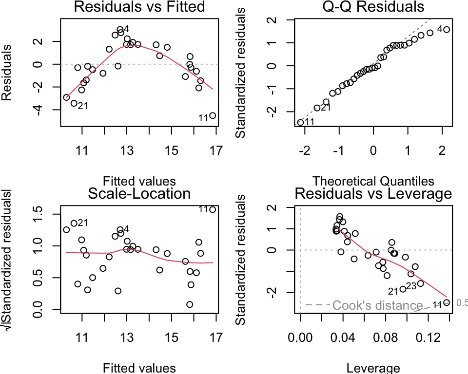
Example: Quadratic Residuals

plot(quadmod)

Exemplary Residual Plot

xx <- runif(500); eps <- rnorm(500); yy = 8 + 6*xx + eps
simfit <- lm(yy~xx); plot(simfit)

Parametric models

• A linear regression model is a type of parametric model; that is lm() assumed a linear functional form for \(f(X)\).

• Parametric models make explicit assumptions about the functional form or distribution of the data.

• Parametric models are characterized by a fixed number of parameters that need to be estimated from the data.

Non parametric models

• Non-parametric models do not assume a specific functional form for the data.

• They are more flexible and do not require a fixed number of parameters.

• Instead of assuming a specific distribution or functional form, non-parametric models rely on the data itself to determine the model’s complexity.

• K-nearest neighbors (KNN) regression, is one such example.

• k-Nearest Neighbors (KNN) is considered a nonparametric model because it makes very few assumptions about the underlying data distribution.
• In contrast to parametric models, which have a fixed number of parameters and assume a specific functional form for the relationship between variables,
• nonparametric models like KNN are more flexible and data-driven.

KNN Regression

Given positive integer \(K\) (chosen by user) and observation \(x_0\):

1. Identify the \(K\) closest points to \(x_0\) in training data. Call this set \(N_0\)
2. Estimate \(f(x_0)\) using \[\begin{equation} \hat f(x_0) = \frac{1}{K} \sum_{i \in N_0} y_i \end{equation}\]

See Ch 7 of Campbell, T., Timbers, T., Lee, M. (2022). Data Science: A First Introduction. United States: CRC Press.

Before $y_i$ was the indicator function counting the number of neighbouring observations beloning to a class. Now we’re simply averaging the neighborhood of y values

Here’s why KNN is classified as nonparametric:

• No Assumed Data Distribution:
• no parameters to be estimated
• No Fixed Model Complexity: Parametric models have a fixed model complexity that is determined by the chosen model structure (e.g., linear, quadratic) and the number of parameters. In KNN, model complexity is not fixed; it can vary depending on the density and distribution of data points in different regions of the feature space. KNN can adapt to both simple and complex patterns in the data.

K = 20

Visualization 1

This is just a step function that takes the closest K=20 points (indicated in red), and averages the corresponding y values

Visualization 2

Animation

K = 5

As K = 5 we get more steps because the averaging over five observations results in much smaller regions of constant prediction

K = 5 Visualization

K = 1

at k=1 we get the most steps with a change occurring at the average between every ordered point.

Conclusion

Small values of \(K\) are more flexible

• produce low bias but high variance
• At \(K=1\) the prediction in a given region is entirely dependent on just one observation.

In contrast, large values of \(K\) are “smoother” with less steps

• less variance (changing one observation has a smaller effect)
• more bias (smoothing masks some of the structure in \(f(X)\))

Again we see the bias-variance trade off in action!

Even when the dimension is small, we might prefer linear regression to KNN from an interpretability standpoint. If the test MSE of KNN is only slightly lower than that of linear regression, we might be willing to forego a little bit of prediction accuracy for the sake of a simple model that can be described in terms of just a few coefficients, and for which p-values are available.

Question: when will a parametric approach such as least squares linear re-gression outperform a non-parametric approach such as KNN regression

Answer: if the parametric form that has been selected is close to the true form of f.