Data 311: Machine Learning

Linear Regression

Dr. Irene Vrbik

University of British Columbia Okanagan

Introduction

• Today we introduce our first model for the supervised regression problem: linear regression.

• Linear regression is a supervised machine learning algorithm used for modeling the relationship between a dependent variable and one or more independent variables by fitting a linear equation to observed data.

• The objective of this model is to find the best-fitting line (or hyperplane) that represents the relationship between the dependent and independent variables.

READ ME

Irene include something about the vif() function to address multicolinearity

Outline

• Why Linear Regression

• Simple linear regression

• Assumptions

• Multiple Linear Regression

• Fitting linear models in R

• Diagnostic Plots

• Measuring Fit

  • \(R^2\) , adjusted \(R^2\), RSE

Any slides in gray you don’t need to pay too much attention to.

Why Linear Regression

• Regression is one of the simplest machine learning algorithms to understand/implement.

Foundational Concept:

It models the relationship between variables in a linear and interpretable way, making it an excellent choice for introductory machine learning courses and for explaining concepts to non-technical stakeholders.

• It provides a solid foundation for learning more complex models and concepts, e.g. model evaluation (MSE), variable selection, overfitting and regularization, \(\dots\)

It helps students and practitioners develop a solid grasp of essential concepts like loss functions, gradient descent, and regularization, which are applicable to many other machine learning algorithms.

checking for multicollinearity, heteroscedasticity, and normality of residuals …

• Linear regression serves as a versatile and widely used benchmark model for many machine learning tasks.

Versatility

It provides a starting point for evaluating the performance of more complex models. If a linear regression model performs reasonably well, it suggests that the relationship between variables is somewhat linear, which can be valuable information.

Motivating Example in Advertising

• The Advertising data set (csv) consists of the sales of a certain product, along with advertising budgets for the product in: TV, radio, and newspaper

• If we establish a link between advertising and sales, we can advise our client to modify their advertising budgets, consequently leading to an indirect increase in sales.

• Our goal is to develop an accurate model that can be used to predict sales on the basis of the three media budgets.

• suppose we are consultants hired to determine if there is an association between advertisting and sales for a product.
• we want to instruct the client on how to adjust advertising budgets (with the goal of indirectly increasing sales)
• IOW we want to develop an accurate model that can be used to predcit sales on the basis of the three media budgets.
• Input (predictions, ind. var, features, “variables”) varials: \(X_1\) = TV, \(X_2\) = Radio, \(X_3\) = Newspaper. Output: sales (response, dependent variable)

The Advertising dataset. The plot displays sales, in thousands of units, as a function of TV, radio, and newspaper budgets, in thousands of dollars, for 200 different markets. In each plot, we show the simple least squares fit of sales to that variable, as described in Chapter 3. In other words, each blue line represents a simple model that can be used to predict sales using TV, radio, and newspaper, respectively.

Motivating Questions

1. Is there an association between advertising and sales ?
2. Which media contribute to sales?
3. How large is the association between each medium and sales?
4. Can we predict Sales using these three?
5. How accurately can we predict future sales?
6. Is the relationship linear?
7. Is there synergy among the advertising media?

These questions can all be tackeled with linear regression. 1. are we wasting our money with advertising? or does it make an impact on sales? 1. Do all three advertising mediums affect sales (just one? two?) how does we tease apart the effect of each when considering all 3 mediums? 1. How much can we expect sales to go up given x amount spent in advertising 1. Not only do we want to give a prediction but we want to know how reliable that prediction is 1. need some diagnostics tools to see if fitting a linear model to this data is even appropriate (we’ll always get an answer out but does it make sense?) 1. synergy is a marketing term indicating that the the whole is greater than the sum of the parts. So perhaps spending 50K on television advertising and 50K on radio advertising is associated with higher sales than allocating $100,000 to either television or radio individually.

synergy refers to the combined effect or interaction of multiple advertising channels that results in a greater impact or effectiveness than the sum of their individual effects.

• It suggests that when different advertising components work together harmoniously, they can amplify the overall impact of an advertising campaign.

  • Consistency across channels to establish brand recognition
  • multiplier effect

Advertising Plots

Below plots the Sales vs TV, Radio and Newspaper, with a blue simple linear-regression line fit separately to each.

ISLR Fig 2.1

ALWAYS PLOT WHEN YOU CAN

• simple plots indicate non-linear behaviour (still seems like this model can be useful)
• wasting money? is gain is sales more than the cost of advertising?
• Left SLR plot ignores radio and newpaper (we can do better than this synergy:

combined effect of multiple predictors on the dependent variable, which can be more significant or different than the sum of their individual effects.

Simple linear regression

We assume that we can write the following model \[Y_i = \beta_0 + \beta_1 X_i + \epsilon_i\]

• \(Y\) is the quantitative response (aka dependent) variable
• \(X\) is the random predictor (aka independent) variable
• \(\beta_0\) is the intercept (unknown)
• \(\beta_1\) is the slope (unknown)
• \(\epsilon\) is the error
• \(i\) is the index for each observation

For simple linear regression (SLR) we only have a single \(X\).

With a single predictor we have “simple” LR

\(\beta_0\) and \(\beta_1\) are parameters (unknown number)

\(X\) are our inputs and \(Y\) and outputs

We know we are not going to be able to predict Y perfectly based on X so we include \(\epsilon\), error term, to account for this mistand.

is a catch-all for what we miss with this simple model:

• the true relationship is probably not linear,
• there may be other variables that cause variation in Y ,
• and there may be measurement error
• natural noise in the data (inherent variability)
• typically assume \(\epsilon \sim N(0, \sigma)\) that the error term is independent of X.

Assumptions

1. Linearity: The relationship between the independent and dependent variables should be (approximately) linear.

The relationship between the independent variables (predictors) and the dependent variable (response) is assumed to be linear.

approximately linear is fine

2. Independence of Errors: The errors (residuals) in the model should be independent of each other.

In other words, there should be no systematic patterns or correlations in the residuals. This assumption is essential to ensure that the model’s predictions are unbiased.

3. Homoscedasticity: the variance of the residuals is constant across all levels of the predictors.

the spread of the residuals should remain roughly the same throughout the range of the independent variables.

2. and 3. can can be summarized as \(\epsilon \sim N(0, \sigma)\)

Notation

For example, \(X_i\) may represent the amount spent in TV advertising in market \(i\), and \(Y_i\) may represent salesof that product in market \(i\). Mathematically, we can write this linear relationship as \[\texttt{sales} \approx \beta_0 + \beta_1 \texttt{TV}\]

Here we “regress sales onto TV”, or we are regressing \(Y\) on \(X\) (or \(Y\) onto \(X\)).

You might read “\(\approx\)” as “is approximately modeled as”.

Multiple Linear Regression

We assume that we can write the following model \[\begin{equation} Y_i = \beta_0 + \beta_1 X_{1,i} + \cdots + \beta_p X_{p,i} + \epsilon_i \end{equation}\]

• \(Y\) is the random, quantitative response variable
• \(X_j\) is the \(j^{th}\) random predictor variable
• \(\beta_0\) is the intercept
• \(\beta_j\) from \(j = 1, \dots p\) are the regression coefficients
• \(\epsilon\) is the error term

For example \(X_1\) may represent TV advertising, \(X_2\) may represent Radio advertising, \(X_3\) may represent Newspaper advertising, and \(Y\) may represent sales. Mathematically, we can write this linear relationship as \[\texttt{sales} \approx \beta_0 + \beta_1 \texttt{TV} + \beta_1 \texttt{Radio} + \beta_e \texttt{Newspaper}\]
Here we regress sales onto the predictors TV, Radio, and Newspaper.

Our SL Model

In terms of our general SL, we have:

\[Y = \beta_0 + \beta_1X_1 + \beta_2X_2 + \ldots + \beta_pX_p\]

• After a model has been selected, we need a procedure that uses the training data to fit or train the model.

• To estimate \(f(X)\), one only needs to estimate the \(p+1\) coefficients \(\beta_0, \beta_1, \ldots, \beta_p\).

• We denote the estimate of \(\beta_i\) by \(\hat \beta_i\).

Fitting the Model

• The most common approach to fitting the linear regression model is referred to as (ordinary) least square, or OLS.

• This least squares technique involves minimizing the sum of the squared residuals, i.e. vertical distance from each point to the line, or curve.

• You can imagine this as wiggling the line about until the sum of the squared vertical distances is minimized.

• This minimization can be achieved using some basic calculus.

OLS is only one of many ways (e.g. gradient descent)

You’ve probably seen this before but i’m going to show this to you under a slightly difference lens ( \(MSE_{train}\) )

Fitted SLR model

Given the parameter estimates \(\hat\beta_0\) and \(\hat\beta_1\) we can predict \(y_i\)
\[\hat y_i = \hat \beta_0 + \hat \beta_1 x_i\]

• \(\hat y_i\) is the estimate of the response variable (some value)
• \(x_i\) is a given predictor variable (some value)
• \(\hat \beta_0\) and \(\hat \beta_1\) is the estimated intercept and slope, respectively.

The least squares regression coefficient estimates (3.4) characterize the least squares line (3.2)

Before we define the residual we need to review some notation.

We use little letters (\(x\), and \(y\)) because they are no longer random variables, but set numbers (e.g. \(x_i\) = 99, \(y_i\) = 10). Similarly, \(\hat\beta\)s are numbers (e.g. \(\hat\beta_0 = 0.04\), \(\hat\beta_1 = 1.1\))

Residuals

• For any line, we can define the observed error as \[e_i = y_i - \hat y_i\] these are more often referred to as residuals.

• To find the “best” line, we instead minimize the residual sum of squares RSS = \(\sum_{i=1}^n e_i^2\).

This is NOT \(\epsilon\)

• \(\epsilon\) = the difference between the observed value and the true model,
• \(e_i\)s are the difference between the observed value and the fitted model

RSS closely mimics the \(MSE_{tr}\) (just missing the numerator).

OLS lm is fit to minimize the \(MSE_{tr}\) (under the model assumptions)

which is reasonable but as we discussed, this does not necessarily mean we’ll have a small \(MSE_{te}\), i.e. it doesn’t guarantee that our model will be generalization to new data

You might be tempted to minimize this error to find the best line, but it can be shown that \(\sum_{i=1}^n e_i = 0\) for any line that passes through the mean of observed \(x\)’s and mean of observed \(y\)’s, ie. through the point ( \(\overline x\), \(\overline y\) )

Estimators

• Derivations for \(\hat \beta_0\) and \(\hat \beta_1\) are easy with some basic calculus (e.g., you can find the derivation for SLR here).

• It turns out that the following equations minimize \(\sum e_i^2\):

\[\begin{align} \hat \beta_1 &= \frac{\sum (y_i - \bar y)(x_i-\bar x)}{\sum (x_i-\bar x)^2}\\ \hat \beta_0 & = \overline{y}- \hat \beta_1\overline{x} \end{align}\]

we won’t be calculating these ourselves. but we will need to know how to extract them from R software

Interpreting Parameter Estimates

• The estimate of intercept, \(\hat \beta_0\), tells us what value we would guess for \(y\) when \(x=0\).

• It is often a large extrapolation¹ (and therefore “meaningless”), so be careful with the interpretation.

• The estimate for slope tells us that for each unit increase in the predictor (\(x\)) we expect the response (\(y\)) to change by \(\hat \beta_1\)

Example of \(\beta_0\) as an extrapolation:

• You are studying the relationship between the number of years of work experience (\(X\)) and annual salary (\(Y\)) for a group of employees.

• You collect data on employees with experience ranging from 5 to 30 years.

If \(\hat \beta_1\) is negative that means \(y\) would decrease as \(x\) increases If \(\hat \beta_1\) is positive that means \(y\) would increase as \(x\) increases

1. Extrapolation is the process of making predictions or estimating values outside the range of the observed data.

Extrapolation

• Suppose researchers want to predict the water retention of the Saguaro cactus at 110°F; however, the observed temperature range in our dataset is only 70°F to 100°F. \[\text{Water retention} = 50 - 0.5 * \text{Temperature} (°F)\]
• Substituting 110°F into the above fitted regression equation suggests that at 110°F, the cactus would have a water retention value of -5 units.

Avoid Extrapolation

Ensure predictions are made within the observed range (i.e. with the range of values in the training data).

Extrapolating to 110 assumes that the same linear relationship holds, which might not be true.

Plugging in blindly could lead to Unreliable Predictions and should be avoided.

that said, we’ll still use \(\beta_0\) (which usually is an extrapolation) and not usually intrept it, but rather consider a parameter to make our model identifiable.

Interpretation for MLR

In MLR we have p predictors; \(X_j\), for \(j = 1, \dots p\).

\(\beta_j\) quantifies the association between the \(j^{th}\) predictor variable and the response.

How do we interpret this?

\(\beta_j\) is the average effect on \(Y\) of a one unit increase in \(X_j\), holding all other predictors fixed

This interpretation is not very useful in practice as predictors will often change together!

for example we might have a fixed budget so spending more on TV advertising would necessarily mean we’d need to spend less in newspaper or radio advertising

Some important questions

1. Is at least one of the predictors \(X_1, X_2, \dots, X_p\)​ useful in predicting the response?

2. Do all the predictors help to explain \(Y\), or is only a subset of the predictors useful?

3. How well does the model fit the data?

4. Given a set of predictor values, what response value should we predict, and how accurate is our prediction?

1. F-test
2. variable selection
3. MSE related values
4. prediction and confidence intervals

Multicollinearity

• Multicollinearity occurs when two or more independent variables in a regression model are highly correlated with each other.

  • e.g., redundant variables (like height in inches and height in centimeters), correlated predictors (e.g. age and years of experience)

• This can lead to unstable coefficient estimates, inflated standard errors, reuduction in overall interpretiblity.

This means that one independent variable can be linearly predicted from the others with a high degree of accuracy.

Coefficient estimates become unstable and sensitive to small changes in the model.

Standard errors of coefficients increase, making it difficult to determine the individual effect of each predictor.

Reduces the overall interpretability of the model, as it becomes challenging to assess the contribution of each variable.

Cars example

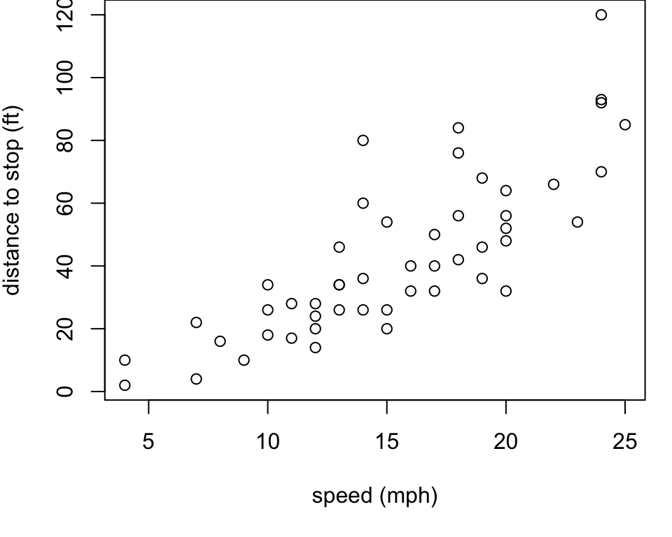
• Let’s consider the cars example from the datasets packages (loaded automatically every time you open R)

• It gives the speed of cars (speed in mph) and the distances taken to stop (dist in ft).

• As a first step, it is always a good idea to plot the data

• Note that the data were recorded in the 1920s.

Cars Plot

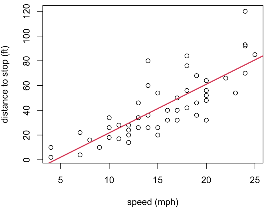
General trend the faster the car is going, the longer (in terms of distance) it takes to stop

Goal find the “best” line to model this trend

lm() function

We fit a linear model in R using the lm() function.

carlm <- lm(dist~speed, data = cars) 

Fitting linear models in R

• If we don’t attach the dataframe, we need to specify the dataframe in the data arguments.

• Alternatively, you could attach() the data set so that the columns in the data frame can be called by name in the lm function.

• Typically, we store the model output in an object and use the summary() function on it to extract more detailed information.

• Clicking on “lm()” in these notes will bring you to their online documentation. To learn more about how summary() works on the output from lm(), use ?summary.lm in R.

You may get a warning of an overwrite here if you already have objects in your R session named dist and speed

Comments

Alternatively we could have attached our data and done the following

attach(cars)
carlm <- lm(dist~speed)

However, this approach is not recommended for this course, as it can lead to confusion when working with different datasets (e.g., training, testing, cross-validation sets).

More generally we will have the following format where a variety of formula specifications are allowed:

fitlm <- lm(formula, data, subset)

Type of model	formula
Single predictor (SLR)	response ~ predictor
Multiple predictors (MLR)	response ~ predictor1 + predictor2 + ...
All variables	response ~ .
Excluding a specific predictor	response ~ . - predictor
Interaction terms	response ~ predictor1 * predictor2
Polynomial terms	response ~ poly(predictor, degree)
Categorical Variables	response ~ factor(predictor)

summary(lm)

summary(carlm)

Call:
lm(formula = dist ~ speed)

Residuals:
    Min      1Q  Median      3Q     Max 
-29.069  -9.525  -2.272   9.215  43.201 

Coefficients:
            Estimate Std. Error t value Pr(>|t|)    
(Intercept) -17.5791     6.7584  -2.601   0.0123 *  
speed         3.9324     0.4155   9.464 1.49e-12 ***
---
Signif. codes:  0 '***' 0.001 '**' 0.01 '*' 0.05 '.' 0.1 ' ' 1

Residual standard error: 15.38 on 48 degrees of freedom
Multiple R-squared:  0.6511,    Adjusted R-squared:  0.6438 
F-statistic: 89.57 on 1 and 48 DF,  p-value: 1.49e-12

talk about the output annotate what is where

Tip

While you should be able to extract this information directly from the summary output, if you want to extract the values from the R object (which is handy for reports) use:

For coefficients

carlm$coefficients

(Intercept)       speed 
 -17.579095    3.932409 

ie carlm$coefficients[2] will renders to: 3.9324088 (\(\hat\beta_1\), the estimate of slope).

For the R-squared value use:

summary(carlm)$r.squared

[1] 0.6510794

(we will discuss what this value represents shortly)

iClicker

iClicker

In linear regression we can have more than one independent variable

A. True

B. False

Correct answer: A. True

iClicker

iClicker

Which term is used to describe the problem when independent variables in a multiple linear regression model are highly correlated?

A. Homoscedasticity

B. Multicollinearity

C. Autocorrelation

D. Heteroscedasticity

Correct answer: B. Multicollinearity

Answer: B) Multicollinearity

Plot OLS line

plot(cars, xlab="speed (mph)", ylab="distance to stop (ft)")
abline(carlm, col=2, lwd= 2)

3D Visualization

ISLR Fig 3.4: In a three-dimensional setting, with two predictors and one response, the least squares regression line becomes a plane. The plane is chosen to minimize the sum of the squared vertical distances between each observation (shown in red) and the plane.

Advertising (SLR)

ISLR Fig 3.1: The least squares fit for the regression of sales onto TV. In this case, a linear fit captures the essence of the relationship, although it is somewhat deficient in the left of the plot

• what do we think about the assumptions here?

Checking Assumptions

Are the assumptions of the linear regression model met?

• linearity

• Normality of residuals

• Homoscedasticity

• Independence

Diagnostic Plots

1. Residuals vs Fitted: checks for linearity. A “good” plot will have a red horizontal line, without distinct patterns.

2. Normal Q-Q: checks if residuals are normally distributed. It’s “good” if points follow the straight dashed line.

3. Scale-Location: checks the equal variance of the residuals. “Good” to see horizontal line with equally spread points.

4. Residuals vs Leverage: identifies influential points¹.

More details about Regression Model Diagnostics at sthda.com.

1. extreme values that might influence the regression results when included or excluded from the analysis.

Diagnostic Plots in R

# plotting options
par(mfrow=c(2,2)) # sets 2x2 layout matrix for plotting
par(mar=c(5,4,1.2,0.1)) # removes some white space around margins

# load in the data
library(dplyr)
Advertising <- read.csv("data/Advertising.csv")
Advertising <- rename(Advertising, market = X) 

# fit the linear regerssion model
adlm <- lm(sales~TV, data = Advertising)

# plot the diagnostic plots
plot(adlm)

Diagnostic Plots in R

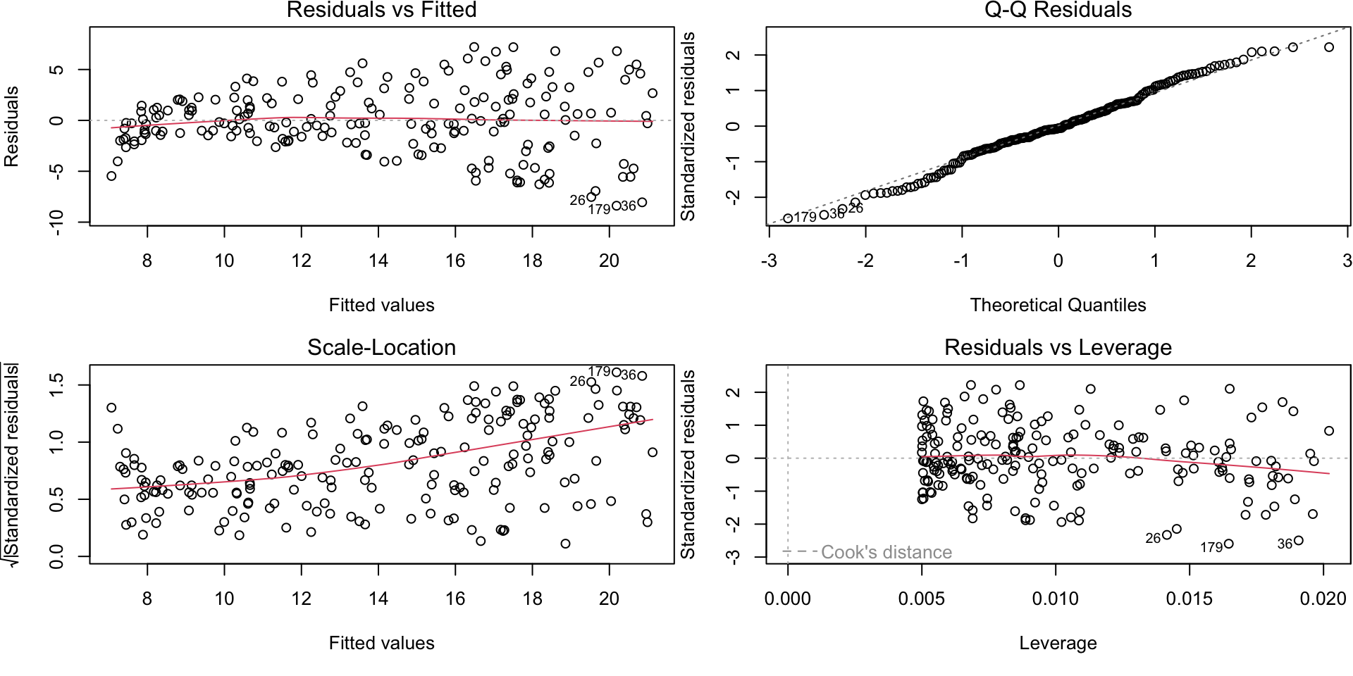
Residuals vs Fitted plot

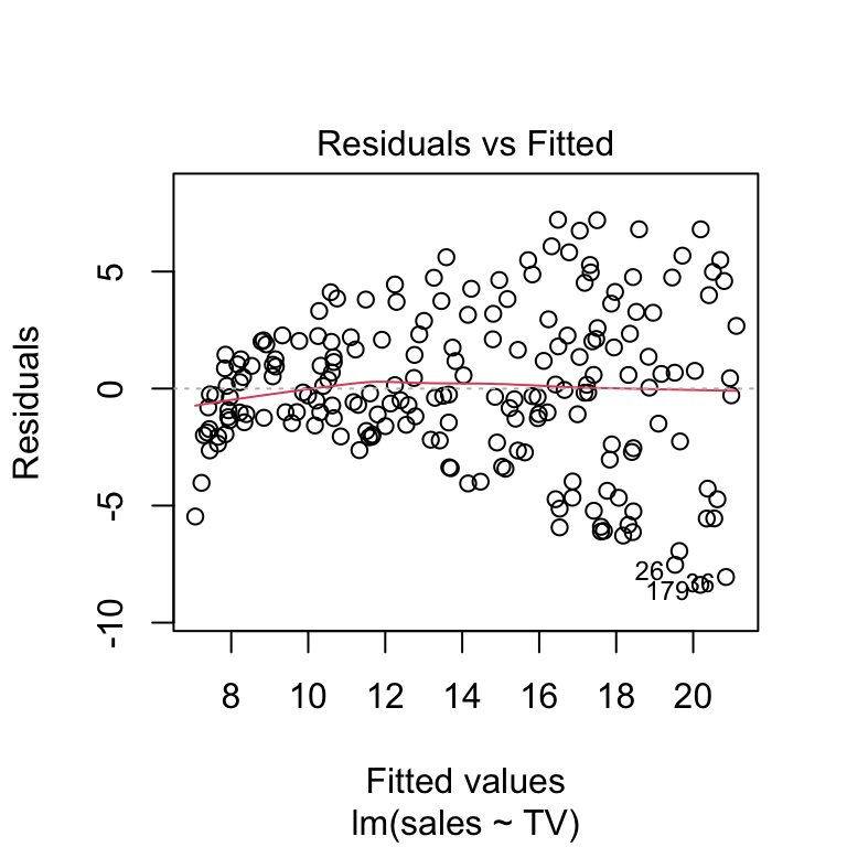
• Purpose: This plot checks for non-linearity, constant variance (homoscedasticity), and the presence of outliers.

• Ideally, the points should be randomly scattered around the horizontal line (y=0), with no clear pattern.

• A systematic pattern (such as a curve) suggests a non-linear relationship, and a “funnel” shape indicates heteroscedasticity (non-constant variance).

Residuals vs Fitted. Used to check the linear relationship assumptions. A horizontal line, without distinct patterns is an indication for a linear relationship, what is good.

1. Residuals vs Fitted: checks for linearity. A “good” plot will have a red horizontal line, without distinct patterns.

Normal Q-Q Plot

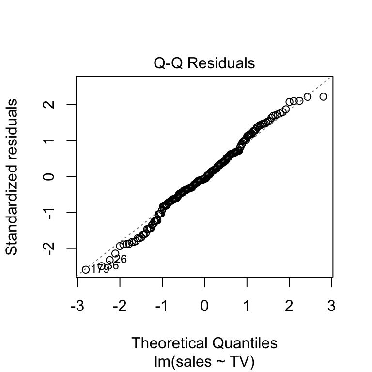
• Purpose: This plot assesses whether the residuals are normally distributed.

• Ideally, the points should lie approximately along the reference line.

• Deviations from this line, particularly in the tails, indicate that the residuals are not normally distributed, which can affect the validity of hypothesis tests and confidence intervals.

Normal Q-Q. Used to examine whether the residuals are normally distributed. It’s good if residuals points follow the straight dashed line.

2. Normal Q-Q: checks if residuals are normally distributed. It’s “good” if points follow the straight dashed line.

Scale-Location Plot

(Spread-Location Plot)

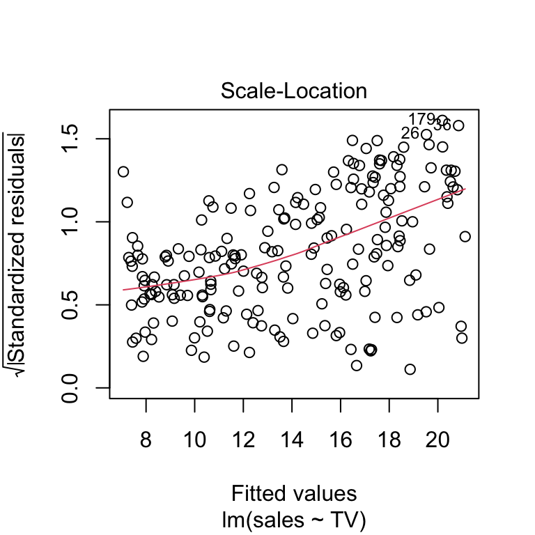
• Purpose: This plot checks for homoscedasticity (constant variance of residuals).

• It plots the square root of standardized residuals against the fitted values.

• Ideally, the points should be scattered horizontally with no discernible pattern. A trend or pattern (e.g., increasing or decreasing spread) suggests heteroscedasticity.

Scale-Location (or Spread-Location). Used to check the homogeneity of variance of the residuals (homoscedasticity).

Horizontal line with equally spread points is a good indication of homoscedasticity. This is not the case in our example, where we have a heteroscedasticity problem.

3. Scale-Location: checks the equal variance of the residuals. “Good” to see horizontal line with equally spread points.

Residuals vs Leverage Plot

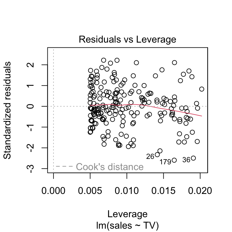
• Purpose: This plot identifies influential observations that have a disproportionate impact on the model fit, also known as high-leverage points.

• It helps to spot influential data points that might unduly affect the regression results.

• Points that are far from others in the x-direction (high leverage) or those with high Cook’s distance (indicated by dashed lines) could be potential concerns.

Residuals vs Leverage. Used to identify influential cases, that is extreme values that might influence the regression results when included or excluded from the analysis.

4. Residuals vs Leverage: identifies influential points¹.

1. extreme values that might influence the regression results when included or excluded from the analysis.

Summary of Assumptions Checked

• Linearity: Assessed through the Residuals vs Fitted plot.
• Normality of Residuals: Assessed through the Normal Q-Q plot.
• Homoscedasticity: Assessed through both the Residuals vs Fitted and Scale-Location plots.
• Independence: Not directly assessed; however, patterns in residuals can indicate problems.

Multicolineartiy problems

Check for correlated variables as they can cause problems

          market    TV  radio newspaper  sales
market     1.000 0.018 -0.111    -0.155 -0.052
TV         0.018 1.000  0.055     0.057  0.782
radio     -0.111 0.055  1.000     0.354  0.576
newspaper -0.155 0.057  0.354     1.000  0.228
sales     -0.052 0.782  0.576     0.228  1.000

• Unstable Coefficient Estimates The variance of all coefficients tend to increase, sometimes dramatically

• Difficulty in Interpreting Coefficients Coefficients may not reflect the true relationship between each predictor and the outcome, leading to misleading conclusions about the importance or impact of each predictor.

newspaper and radio are highly correlated which can lead to unstable and unreliable estimates of the regression coefficients. Can also lead to higher error

IF there is high correlation you might consider removing one of those variables

alternatively we could look at functions like the vif() from the car package to Variance Inflation Factor (VIF) measures how much the variance of a regression coefficient is inflated due to multicollinearity with other predictors.

You will see in lab that as soon as you start removing correlated predictors these coefficeints are going to change dramatically.

Looking Forward

• To deal with correlated variables you may consider removing one of the highly correlated predictors (you will look at a technique called backward selection in the lab)

• Alternatively, you could combine correlated predictors into a single composite variable (we don’t cover this here).

• Regularization methods add a penalty to the regression model to shrink coefficient estimates and reduce multicollinearity effects (we will look at Ridge Regression and Lasso in future lectures)

Assessing the Accuracy of the Coefficient Estimates

The standard error of an estimator reflects how it varies under repeated sampling. We have \[\begin{align*} SE(\hat{\beta}_1)^2 &= \frac{\sigma^2}{\sum_{i=1}^{n}(x_i - \bar{x})^2},\\ SE(\hat{\beta}_0)^2 &= \sigma^2 \left(\frac{1}{n} + \frac{\bar{x}^2}{\sum_{i=1}^{n}(x_i - \bar{x})^2}\right), \end{align*}\] where \(\sigma^2 = \text{Var}(\epsilon)\).

sigma

• The \(\sigma\) used in the standard error formula represents the standard deviation of the error terms, ie. \(\sigma^2 = \text{Var}(\epsilon_i)\)

• Since \(\sigma\) is generally unknown and is estimated with \[\begin{equation} RSE=\sqrt{\frac{RSS}{n-p-1}} = \sqrt{\frac{\sum (Y_i-\hat{Y}_i)^2}{n-p-1}} \end{equation}\]

• This estimate stands for the residual standard error and serves as a measure of the amount of training error in the model (we’ll come back to this later)

Confidence Intervals

• These standard errors can be used to compute confidence intervals.
• A 95% confidence interval is defined as a range of values such that with 95% probability, the range will contain the true unknown value of the parameter.
• It has the form

\[\hat{\beta}_1 \pm 1.96 \cdot SE(\hat{\beta}_1)\]

Confidence intervals (continued)

That is, there is approximately a 95% chance that the interval

\[[\hat{\beta}_1 - 1.96 \cdot SE(\hat{\beta}_1), \hat{\beta}_1 + 1.96 \cdot SE(\hat{\beta}_1)]\]

will contain the true value of \(\beta_1\) (under a scenario where we get repeated samples like the present sample). For the advertising data, the 95% confidence interval for \(\beta_1\) is \[[0.042, 0.053]\]

Confidence interval in R

Advertising <- read.csv("https://www.statlearning.com/s/Advertising.csv")
adlm <- lm(sales~TV, data = Advertising)
sumlm <- summary(adlm)
# Confidence interval for the coefficient of TV
beta_tv <- sumlm$coefficients["TV", c("Estimate", "Std. Error")]

# Calculate the critical value (two-tailed)
alpha <- 0.05
n <- nrow(Advertising)
critical_value <- qt(1 - alpha / 2, df = n - length(adlm$coefficients))

# Calculate the lower and upper bound of the CI
lower_bound <- beta_tv["Estimate"] - critical_value * beta_tv["Std. Error"]
upper_bound <- beta_tv["Estimate"] + critical_value * beta_tv["Std. Error"]
print(c(lower_bound, upper_bound))

  Estimate   Estimate 
0.04223072 0.05284256 

Hypothesis Testing

• Standard errors can also be used to perform hypothesis tests on the coefficients.
• The most common hypothesis test involves testing

\[\begin{align} H_0: & \text{ There is no relationship between $X$ and $Y$ vs. }\\ H_A: & \text{ There is some relationship between $X$ and $Y$}. \end{align}\]

• Mathematically, this corresponds to testing \(H_0: \beta_1 = 0\) versus \(H_A: \beta_1 \neq 0\), since if \(\beta_1 = 0\), then the model reduces to \(Y = \beta_0\), and \(X\) is not associated with \(Y\).

we’ll skip through this as this is part of your pre-reqs but note that after we reject the null we can go onto the next step

Hypothesis testing for multiple linear regression

In the multiple regression setting with \(p\) predictors, we need to ask whether all of the regression coefficients are zero, i.e., whether \[\beta_1 = \beta_2 = \ldots = \beta_p = 0.\]

To answer this question we test the null hypothesis, \[\begin{align*} H_0:& \beta_1 = \beta_2 = \ldots = \beta_p = 0 \\ H_a:& \text{at least one } \beta_j \text{ is non-zero} \end{align*}\]

F-test

This hypothesis test is performed by computing the F-statistic where \(F\) follows an \(F\)-distribution with degrees of freedom \(\nu_1 = p\) and \(\nu_2 = n-p-1\)

\[\begin{equation} F = \frac{\text{TSS - RSS}/p}{\text{RSS}/(n - p - 1)} \end{equation}\]

If there is no relationship between the response and predictors, the F-statistic will be close to 1. Larger values produce smaller p-values and a higher chance of rejecting \(H_0\).

these hypothesis tests (along with diagnostic checks) should be done before you move to assessment

as with simple linear regression, TSS = \((y_i - \bar{y})^2\) and RSS = \((y_i - \hat{y}_i)^2\).

Measuring Fit

• Once we have determined that it is likely that there is a significant relationship between \(X\) and \(Y\), we can ask: how well does the linear model fit the data?

• You may remember assessing the quality of a linear regression fit using the following methods

  1. the coefficient of determination, or \(R^2\) statistic (and adjusted \(R^2\) for multiple linear regression)
  2. the residual standard error (RSE)

• we already discussed rse: provides an absolute measure of lack of fit
• since it is measured in the units of Y, it is not always clear what constitutes a “good” RSE.
• \(R^2\) serves as an alternative measure that always falls between 0 and 1 (independent of the scale of Y). unlike RSE the bigger the better.

R-squared

\[\begin{equation} R^2 = \frac{\text{TSS-RSS}}{\text{TSS}} = 1-\frac{\text{RSS}}{\text{TSS}} = 1- \frac{\sum (y_i - \hat y_i)^2}{\sum (y_i - \bar y)^2}. \end{equation}\]

• The coefficient of determination \(R^2\) is the proportion of the total variation that is explained by the regression line.

• It measures how close the fitted line is to the observed data.

• It is easily to interpret as it always lies between 0 and 1

• tss is the residuals of the null model
• in SLR: Hence, R2 measures the proportion of variability in Y that can be explained using X.
• High R2 → a large proportion of the variability in the response is explained by the regression.
• Low R2 → the regression does not explain much of the variability in the response.

Pros:

Interpretability: It is easy to interpret and understand: x% of the variance in the response variable is explained by the model.

Scale Independence: It is unitless and not dependent on the scale of the response variable, making it useful for comparing models with different response variables.

CONS

Does Not Reflect Fit Quality: can be artificially high due to overfitting or when irrelevant variables are added.

Where TSS is the total sum of squares = \(\sum_{i=1}^{n}(y_i - \bar{y})^2\) and RSS are the residual sum of squares \(\sum (y_i - \hat y_i)^2\). It is supplied in the summary(lm) output, see cars example

Adjusted \(R^2\)

Adjusted \(R^2\) is produced in R output and calculated by:

\[ R^2 = 1 - \dfrac{\dfrac{RSS}{n-p-1}}{\dfrac{TSS}{n-1}} \]

• This metric penalizes for over-parameterization¹
• Goodness of fit measure (bigger = better)

We usually look at adjusted \(R^2\) when comparing models with different number of predictors

• adjusts for the number of predictors in the model.
• increases when the new term improves the model more than would be expected by chance.
• relates to MSE_training always improving as we increase model complexity
• it decreases when a predictor improves the model by less than expected.
• it is always lower than the R-squared.

There are other metrics, eg AIC, BIC, Mallows’ \(C_p\)

1. involves adding more predictors, features, or parameters to a model than what is justified or needed.

RSE

RSE is calculated as follows:

\[\begin{equation} RSE = \sqrt{\frac{1}{n - p - 1} \sum_{i=1}^{n} (y_i - \hat{y}_i)^2}\end{equation}\]

where \(n\) is the number of data points, \(p\) is the number of predictors (features), \(y_i\) is the observed value, and \(\hat y_i\)​ is the predicted value for the \(i^{th}\) data point.

Does this formula remind you of anything? \(MSE = \frac{1}{n} \sum_{i=1}^{n} (y_i - \hat{y}_i)^2\)

• When \(p\) (the number of predictors) is small relative to \(n\) (the number of data points), RSE and MSE will be similar.
• However, as the number of predictors increases relative to the sample size, RSE will tend to be larger than MSE due to the degrees of freedom adjustment.

Recall the standard deviation calculation \(SD = \sqrt{\frac{\sum_{i=1}^n (x_i - \bar{x})^2}{n - 1}}\)

RSE (continued)

• RSE is primarily used in the context of linear regression.

• It quantifies the typical or average magnitude of the residuals (the differences between observed and predicted values) in the model.

RSE is essentially the standard deviation of the residuals \(\left(\sqrt{\text{Var}(e_i)}\right)\).

RSE is used to estimate \(\sigma\) the standard error of errors \(\left(\sqrt{\text{Var}(\epsilon)}\right)\)

bigger the \(\sigma\) the more spread out the points are around the line

Lower RSE or RMSE values indicate better model accuracy. These metrics give you a sense of how well the model’s predictions match the actual data points.

Pros:

Direct Interpretation: It is in the same units as the response variable, making it easy to interpret. A lower RSE indicates a better fit.

Useful for Absolute Fit: It gives a sense of the absolute fit of the model. If RSE is very small, it means the model fits the data very well.

Cons:

Scale Dependent: RSE depends on the units of the response variable, making it hard to compare across models with different response variables.

Does Not Directly Indicate Proportion of Variance Explained: Unlike \(R^2\) , it doesn’t directly indicate how much variance is explained by the model.

RSE vs. MSE

Recall our Mean Squared Error (MSE) formula from last lecture:

\[ MSE = \frac{1}{n} \sum_{i=1}^{n} (y_i - \hat{y}_i)^2 \]

• MSE is a more general metric used in various machine learning and statistical modeling contexts

• RSE is essentially a scaled version of MSE.

• RSE is a specific metric used in linear regression that adjusts for the number of predictors, whereas MSE is a more general metric used in various predictive modeling tasks.

• MSE is not limited to linear regression unlike \(R^2\) and RSE
• When \(p\) (the number of predictors) is small relative to \(n\) (the number of data points), RSE and MSE will be similar.
• However, as the number of predictors increases relative to the sample size, RSE will tend to be larger than MSE due to the degrees of freedom adjustment. \[\sqrt{\frac{1}{n - p - 1} \sum_{i=1}^{n} (y_i - \hat{y}_i)^2}\]
• MSE=(1−R2)×Var(Y) for simple linear regression
• However, in multiple linear regression (with multiple predictors), the relationship between MSE and \(R^2\) becomes more complex due to the additional predictors. A decrease in MSE may or may not lead to an increase in \(R^2\) because the model’s fit can improve with more predictors even if the prediction error (MSE) remains the same.

Example: Life Expectancy (SLR)

• Lets consider a data set containing the life expectancy and illiteracy rates (among other measurements) for all 50 states from the 1970’s.

• This dataset is available in R as state.x77 in the datasets package (which gets loaded automatically with each new R session), see ?state.x77

• We’ll fit a simple linear regression with life expectancy Life.Exp¹ as the response variable.

1. we have renamed the columns of this data set and replaced spaces with periods

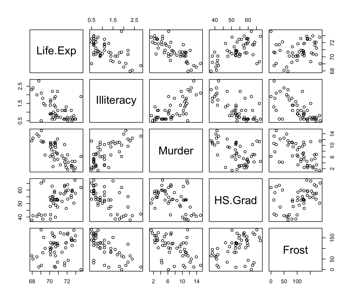
Example: Life Expectancy (MLR)

Our response variable is Life.Exp the life expectancy in years (1969–71). Lets consider the predictors:

• Illiteracy: illiteracy (1970, percent of population)
• Murder: murder and non-negligent manslaughter rate per 100,000 population (1976)
• HS Grad: percent high-school graduates (1970)
• Frost: mean number of days with minimum temperature below freezing (1931–1960) in capital or large city

use some common sense - should frost impact the life expectancy? Should colder places result in people living shorter? maybe or maybe this is a confounding variable that is masking the read underlying cause (less crime in winter)

I have changed the variable names to remove spaces

Scatterplot

• A pairs plot allows us to see both distribution of single variables and relationships between two variables.
• Every variable constitutes 1 row and 1 column of our pairs matrix. For example, row 2 and column 1 corresponds to the scatterplot and correlation between Illiterarcy and Frost.
• correlation does not imply causation!!
• Some more examination will be required to be done once significant variables are obtained for linear regression modeling. (with help of residual plots, the coefficient of determination i.e Multiplied R square we can reach closer to our results) [1]

SLR in R with Illiteracy

fit1 <- lm(Life.Exp~Illiteracy, data= stdata)
summary(fit1)

...
Call:
lm(formula = Life.Exp ~ Illiteracy, data = stdata)

Coefficients:
            Estimate Std. Error t value Pr(>|t|)    
(Intercept)  72.3949     0.3383 213.973  < 2e-16 ***
Illiteracy   -1.2960     0.2570  -5.043 6.97e-06 ***
---
Signif. codes:  0 '***' 0.001 '**' 0.01 '*' 0.05 '.' 0.1 ' ' 1

Residual standard error: 1.097 on 48 degrees of freedom
Multiple R-squared:  0.3463,    Adjusted R-squared:  0.3327 
F-statistic: 25.43 on 1 and 48 DF,  p-value: 6.969e-06
...

iClicker

iClicker coefficient

What is the coefficient of Illiteracy?

1. 72.39

2. -1.3

3. 0.35

4. 0.33

5. None of the above

Correct answer: B

iClicker p-value

What is the \(p\)-value associated with the coefficient of Illiteracy?

1. 3.47e-73

2. 6.97e-06

3. 213.97

4. -5.04

5. None of the above

Correct answer: B

Illiteracy Coefficient: -1.2960, meaning an increase in illiteracy by one unit is associated with a decrease in life expectancy by approximately 1.3 years on average.

iClicker lm output

iClicker: p-value associated with regression coefficients

What does the p-value associated with the Illiteracy coefficient represent?

1. The probability that Illiteracy has no effect on Life Expectancy.

2. The proportion of Life Expectancy variance explained by Illiteracy

3. The probability of observing the estimated relationship between Illiteracy and Price, or something more extreme, if Illiteracy had no impact on Life Expectancy.

4. The change in Life Expectancy for each additional unit of Illiteracy

Correct Answer: C

the solo affect of illiteracy does seem to be a significant predictor (very small p-value) strong evidence of a linear relationship between life expectancy and age

SLR with Illiteracy

• Illiteracy Coefficient: \(\hat \beta_{1}\) = -1.3 \(\rightarrow\) a 1% increase in illiteracy is associated with a decrease in life expectancy by approximately -1.3 years on average.

• The R-squared value 0.35 suggests that Illiteracy explains around 35% of the variance in life expectancy.

• Residual Standard Error (RSE): 1.097, indicating the average distance of observed values from the regression line.

rse <- summary(fit1)$sigma # RSE is stored as sigma

Notice how i don’t just use generic “one unit increase”

For SLR we look at R^2 for it’s nice interpretation.

Note the highly significant \(p\)-value of 3.47e-73.

SLR in R with Frost

frost.fit <- lm(Life.Exp~Frost, data= stdata)
(sff <- summary(frost.fit))

Call:
lm(formula = Life.Exp ~ Frost, data = stdata)

Residuals:
    Min      1Q  Median      3Q     Max 
-2.6515 -0.7852 -0.1183  0.9382  3.4284 

Coefficients:
             Estimate Std. Error t value Pr(>|t|)    
(Intercept) 70.171631   0.418883 167.521   <2e-16 ***
Frost        0.006768   0.003597   1.881    0.066 .  
---
Signif. codes:  0 '***' 0.001 '**' 0.01 '*' 0.05 '.' 0.1 ' ' 1

Residual standard error: 1.309 on 48 degrees of freedom
Multiple R-squared:  0.06868,   Adjusted R-squared:  0.04928 
F-statistic:  3.54 on 1 and 48 DF,  p-value: 0.06599

SLR with Frost

• The weak positive relationship (\(\hat \beta_{\text{Frost}}\) = 0.0068) between Frost and Life Expectancy is not significant (\(p\)-value = 6.60e-02.

• This suggests that there is no strong evidence of a relationship between the number of frost days and life expectancy.

MLR in R

summary(fit2 <- lm(Life.Exp~Illiteracy+Murder+HS.Grad+Frost, data= stdata))

Call:
lm(formula = Life.Exp ~ Illiteracy + Murder + HS.Grad + Frost, 
    data = stdata)

Residuals:
     Min       1Q   Median       3Q      Max 
-1.48906 -0.51040  0.09793  0.55193  1.33480 

Coefficients:
             Estimate Std. Error t value Pr(>|t|)    
(Intercept) 71.519958   1.320487  54.162  < 2e-16 ***
Illiteracy  -0.181608   0.327846  -0.554  0.58236    
Murder      -0.273118   0.041138  -6.639  3.5e-08 ***
HS.Grad      0.044970   0.017759   2.532  0.01490 *  
Frost       -0.007678   0.002828  -2.715  0.00936 ** 
---
Signif. codes:  0 '***' 0.001 '**' 0.01 '*' 0.05 '.' 0.1 ' ' 1

Residual standard error: 0.7483 on 45 degrees of freedom
Multiple R-squared:  0.7146,    Adjusted R-squared:  0.6892 
F-statistic: 28.17 on 4 and 45 DF,  p-value: 9.547e-12

talk about r syntax

Hypothesis test

• We want to know if our predictors are useful in predicting life expectancy (our response variable Life.Exp)

• We could first test if any of the predictors under consideration are significant. Namely, we test

\[\begin{align} H_0&: \beta_1 = \beta_2 = \cdots = \beta_p = 0 && H_a: \text{not all }\beta_j = 0 \end{align}\]

• This is conducted using the \(F\)-test…

F test

summary(fit2)

Call:
lm(formula = Life.Exp ~ Illiteracy + Murder + HS.Grad + Frost, 
    data = stdata)

Residuals:
     Min       1Q   Median       3Q      Max 
-1.48906 -0.51040  0.09793  0.55193  1.33480 

Coefficients:
             Estimate Std. Error t value Pr(>|t|)    
(Intercept) 71.519958   1.320487  54.162  < 2e-16 ***
Illiteracy  -0.181608   0.327846  -0.554  0.58236    
Murder      -0.273118   0.041138  -6.639  3.5e-08 ***
HS.Grad      0.044970   0.017759   2.532  0.01490 *  
Frost       -0.007678   0.002828  -2.715  0.00936 ** 
---
Signif. codes:  0 '***' 0.001 '**' 0.01 '*' 0.05 '.' 0.1 ' ' 1

Residual standard error: 0.7483 on 45 degrees of freedom
Multiple R-squared:  0.7146,    Adjusted R-squared:  0.6892 
F-statistic: 28.17 on 4 and 45 DF,  p-value: 9.547e-12

Any weird here?

iClicker F test

iClicker: What is the \(p\)-value associated with F-test

What does the p-value associated with the F test?

1. < 2e-16
2. 5.82e-01
3. 3.50e-08
4. 1.49e-02
5. 9.547e-12

Correct Answer: e: 9.547e-12

Interpretation

The \(p\)-value of the F-statistic is highly significant which means that, at least, one of the predictor variables is significantly related to the outcome variable.

scroll down to see a really small p-value

We saw those sums of squares in our \(R^2\) (coefficient of determiniation calculations).

It can be shown if the linear model assumptions are correct,

• the expectation of the denominator is \(\sigma^2\)
• (+provided \(H_0\) is true) the expectation of the numerator is \(\sigma^2\) Hence [PRESS ENTER] where there is no relationship between the response and predictors one would expect the F-statisitcs to take on a value close to 1. - why too much info need to know SS* and DF* formulas

Comments on the F-test

Q: Why do we use F-tests instead of looking at the individual p-values associated with each predictor?

• Even if all \(\beta_j\)’s = 0, (that is, no variable is truly associated with the response), we would still expect 5% of hypothesis tests for \(\beta_j\) to be rejected by chance alone

• The \(F\)-test therefore combats the multiple testing problem.

  Warning

  If \(p>n\) we cannot fit MLR model using least squares.

Hence, if H0 is true, there is only a 5% chance that the F-statistic will result in a p- value below 0.05, regardless of the number of predictors or the number of observations. - there are some tricks we can use (discussed later) including forward and backward selection

1. Is at least one predictor useful?

• For that question, we use the F-statistic and F-test

• Since the value is large (28.17) and the p-value is small (9.547e-12) we would reject the null \[H_0: \beta_0 = \beta_1 = \beta_2 = \beta_3\] in favour of the alternative

\[ H_a:\text{ at least one }\beta_j \neq 0. \]

2. Do all the predictors help to explain \(Y\), or is only a subset of the predictors useful?

• Each \(\beta_j\) has an associated \(t\)-statistic and \(p\)-value in the R output

• These check whether each predictor is linearly related to the response, after adjusting for all the other predictors considered

• These are useful, but we have to be careful…especially for large numbers of predictors (multiple testing problem)

• (hence the lack of stability when fitting different numbers of predictors).
• (because of the compounding error rates, we would expect to see variables meet our significance level threshold by chance).

Attempt no. 1

• A natural temptation when considering all these individualized hypothesis tests is to “toss out” any variable(s) that does not appear significant (ie \(p\)-value > 0.05)

• This brings us into the topic of variable selection, which we will go into much more detail later in the course.

• As our first foray, we’ll look at the most straightforward (and also oldest) techniques for doing so.

• this is flawed since coefficient in combination with different predictors may or not be significant
• so b2 might be significant when x4 and x6 are in the model, but not significant when x5 and x2 are in the model.
• so there is so instability in these values We will look at some other clever ways of performing variable selection later on in the course

Attempt no. 2

• Assuming we now have an appropriate measuring stick (e.g. RSE or \(R^2\)) how do we go about choosing which models to fit?

• Ideally we would try every combination of \(X_j\), but that becomes computationally impractical very quickly¹

• Instead, we may decided on a systematic approach to perform model selection: …

1,073,741,824 over 1 billion combinations

1. there are over a million two-predictor models when \(p=30\), \(2^{30} = 1.0737418\times 10^{9}\)

Variable Selction

• Forward Selection: Start with only the intercept (no predictors, ie null model). Create \(p\) simple linear regressions, whichever predictor has the lowest RSS, add it into the model. Continue until, for instance, we see a decrease in our ‘best model’ measurement.

• Backward Selection: Start with all predictors. Remove the predictor with the largest p-value. Continue until, for instance, all variables are considered significant.

• Mixed Selection: Start with no predictors. Perform forward selection, but if any \(p\)-values for variables currently in the model reach above a threshold, remove that variable. Continue until, for instance, all variables in your model are significant and any additional variable would not be.

• Backward selection cannot be used if p > n, while forward selection can always be used.
• Forward selection is a greedy approach, and might include variables early that later become redundant. Mixed selection can remedy this.
• You will consider regularization approaches that get around this issue later in the course
• mixed if at any point the p-value for one of the variables in the model rises above a certain threshold, then we remove that variable from the model.

Types of Error

We are always going to encounter error by using models.

1. Because we are estimating the population parameters \(\beta_j\) based on a sample there will always be some variability in our model and inaccuracy related to the reducible error.

2. Our model will most likely be a simpler approximation to reality hence, we introduce model bias and add to our reducible error

3. Even if the multiple linear model was exactly \(f\), there would still be irreducible error. That is, our predictions \(\hat y_i \neq y_i\) for most (probabilistically all) \(i\).

• are there variables we could have collected but didn’t that could have improved our model?
• did we select the best subset among the ones we did record?
• We operate under the assumption that our model is not overtly biased (since this is not measurable in realistic circumstances).

3. How well does the model fit the data?

• While the summary() function does not spit out the MSE by default, we can still calculate this value and compre the resulting MSE with the MSE of other fitted models using the same data.

• That is to say the MSE isn’t so useful on it’s own but more-so as a comparative value across multiple models.

4. Given a set of predictor values, what response value should we predict, and how accurate is our prediction?

• We can use the fitted model to make predictions for \(Y\) on the basis of a set of predictors \(X_1, X_2, \dots, X_p\) using functions in R and the fitted \(\hat \beta\)’s

• To account for the three sorts of uncertainty associated with this prediction we have two methods:

  1. confidence intervals: reflects the uncertainty around the mean prediction values.
  2. prediction intervals: reflects the uncertainty around a single value

Prediction a single value

• Using the SLR model for the cars data, we can predict the stopping distance for a new speed value \(x_0\).

• Its stopping distance will be determined by \[Y_0 = \beta_0 + \beta_1 x_0 + \epsilon\]

• Our prediction for this value would be \(\hat\beta_0 + \hat\beta_1 x_0\)

• To assess the variance of this prediction, we must take into account the variance of the \(\hat\beta\)s and \(\epsilon\).

Prediction a mean response

• Suppose we are interested in the average stopping distance this 1920s car would incur at a speed of \(x_0\).

• Our prediction for this value would be \[\hat y_0 = \hat\beta_0 + \hat\beta_1 x_0\]

• To assess the variance of this prediction, we only need to take into account the variance of the \(\hat\beta\)s.

Predict the average outcome rather than a single outcome

Making Predictions

• Prediction intervals are concerned with the value of a new observation \(Y_{0}\) for a given value \(x_0\) of the predictor

• Confidence intervals are concerned with the value of the mean response \(E(Y_0) = \mu_{Y_0}\) for a given value \(x_0\) of the predictor

• Prediction intervals are more commonly required as we are often interested in predicting an individual value

Confidence intervals the mean response are less commonly sought after

You will look at how to do this using the predict() function in lab.

Pros

Simplicity: easy to understand, interpret and implement.

Efficiency: It is computationally inexpensive, trains very quickly compared to more complex models, especially on smaller datasets.

Baseline Model: serves as a good baseline model for more complex techniques, helping to determine if further sophistication is necessary.

Predictive Power: if the relationship between the variables is truly linear, it can produce highly accurate predictions.

Cons

Strong Assumptions: assumes assumptions is violated, the model may not perform well.

Limited to Linear Relationships: underfits when applied to complex relationships.

Sensitivity to Outliers: highly sensitive to outliers, which can disproportionately affect the model’s accuracy.

Multicollinearity: When independent variables are highly correlated, linear regression coefficients can become unstable and misleading.

It provides a clear mathematical relationship between the independent variables and the dependent variable.

Interpretability: The coefficients of the model can be easily interpreted to understand the influence of each independent variable on the dependent variable.

Most software will support model fitting (eg excel, ggplot plotting features can easily superimpose a linear regression model).

Homoscedasticity Assumption: Linear regression assumes constant variance in the error terms. Violating this assumption can lead to inaccurate estimates and invalid inferences.

Looking Forward

• In this weeks lab, you cover how to fit SLR and MLR in R using a training set, and assess them on a test set.
• We will look at some extension to the linear regression model that will make them more flexible.
• Look at an non-parametric alternatives for regression problems (more flexible).
• For more practice, go through ISLR 3.6 Lab: Linear Regression