library(glmnet)Loading required package: MatrixLoaded glmnet 4.1-8Regularization Methods
In this lab we discuss a few ways in which the linear model may be improved in terms of prediction accuracy and model interpretability. These methods will be particularly using in scenarios where \(n < p\)
Ridge Regression and LASSO are regularization techniques that are used in linear regression models to tackle the \(n<p\) problem and improve model performance. In addition, these methods could be useful to address the issues of multicollinearity and overfitting.
They work by constraining or “shrinking” the estimated coefficients toward zero, but it does not set coefficients exactly to zero. By doing this we can often substantially reduce the variance at the cost of a negligible increase in bias.
Ridge Regression adds a regularization term (L2 regularization) to the linear regression cost function. In other words, there is a “budget” on how large \(\sum_j = 1^p \beta_j\) can thereby penalizing the absolute magnitude of regression coefficients.
Similar to Ridge Regression, LASSO adds a regularization term (L1 regularization) to the linear regression cost function. Put simply, it penalizes the number of non-zero coefficients. LASSO tends to shrink some coefficients all the way to zero, effectively performing variable selection by eliminating some features from the model. By removing these variables—that is, by setting the corresponding coefficient estimates to zero—we can obtain a model that is more easily interpreted.
Both of these models can be fit using glmnet() from the package of the same name.
library(glmnet)Loading required package: MatrixLoaded glmnet 4.1-8Usage
glmnet(x, y, family = c("gaussian", "binomial", "multinomial"),
alpha = 1, nlambda = 100)alpha = 0 we get Ridge Regressionalpha = 1 we get LASSOlambda is the size of the penalty. By default the glmnet() will automatically selected range of \(\lamda\) values.NOTE: by default variables are standarized so that they are on the same scale.
Let’s recreate the simulations from lecture. We assume the predictors are normally distributed (with differing means and standard deviations) and the response is assumed \(Y=20 + 3X_1 - 2X_2 + \epsilon\) where epsilon is normal \((\mu=0, \sigma^2=4)\)
set.seed(35521)
x1 <- rnorm(30,0,3)
x2 <- rnorm(30,1,4)
y <- 20 + 3*x1 - 2*x2 + rnorm(length(x1), sd=2)
x <- cbind(x1, x2)
pairs(cbind(y,x))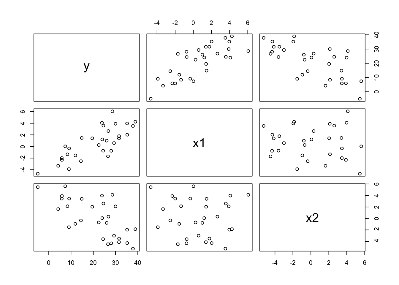
Now we fit a standard linear model to see how close we are to estimating the true model…
linmod <- lm(y~x1+x2)
summary(linmod)
Call:
lm(formula = y ~ x1 + x2)

Residuals:
    Min      1Q  Median      3Q     Max
-4.7524 -0.9086 -0.1260  1.7005  3.0130

Coefficients:
            Estimate Std. Error t value Pr(>|t|)
(Intercept)  19.4425     0.3636   53.47   <2e-16 ***
x1            3.0808     0.1335   23.07   <2e-16 ***
x2           -2.1267     0.1097  -19.39   <2e-16 ***
---
Signif. codes:  0 '***' 0.001 '**' 0.01 '*' 0.05 '.' 0.1 ' ' 1

Residual standard error: 1.941 on 27 degrees of freedom
Multiple R-squared:  0.9734,    Adjusted R-squared:  0.9714
F-statistic: 494.4 on 2 and 27 DF,  p-value: < 2.2e-16
Now ridge regression…
rrsim_d <- cv.glmnet(x, y, alpha=0)
plot(rrsim_d$glmnet.fit, label=TRUE, xvar="lambda")
plot(rrsim_d)
rrsim_d$lambda.min[1] 0.8770535Since the minimum was determined nearly at the lower boundary of \(\lambda\), it’s worthwhile to try a different grid of \(\lambda\) values than what the default provides…
grid <- exp(seq(10, -6, length=100))
set.seed(451642)
rrsim <- cv.glmnet(x, y, alpha=0, lambda=grid)
plot(rrsim$glmnet.fit, label=TRUE, xvar="lambda")
plot(rrsim)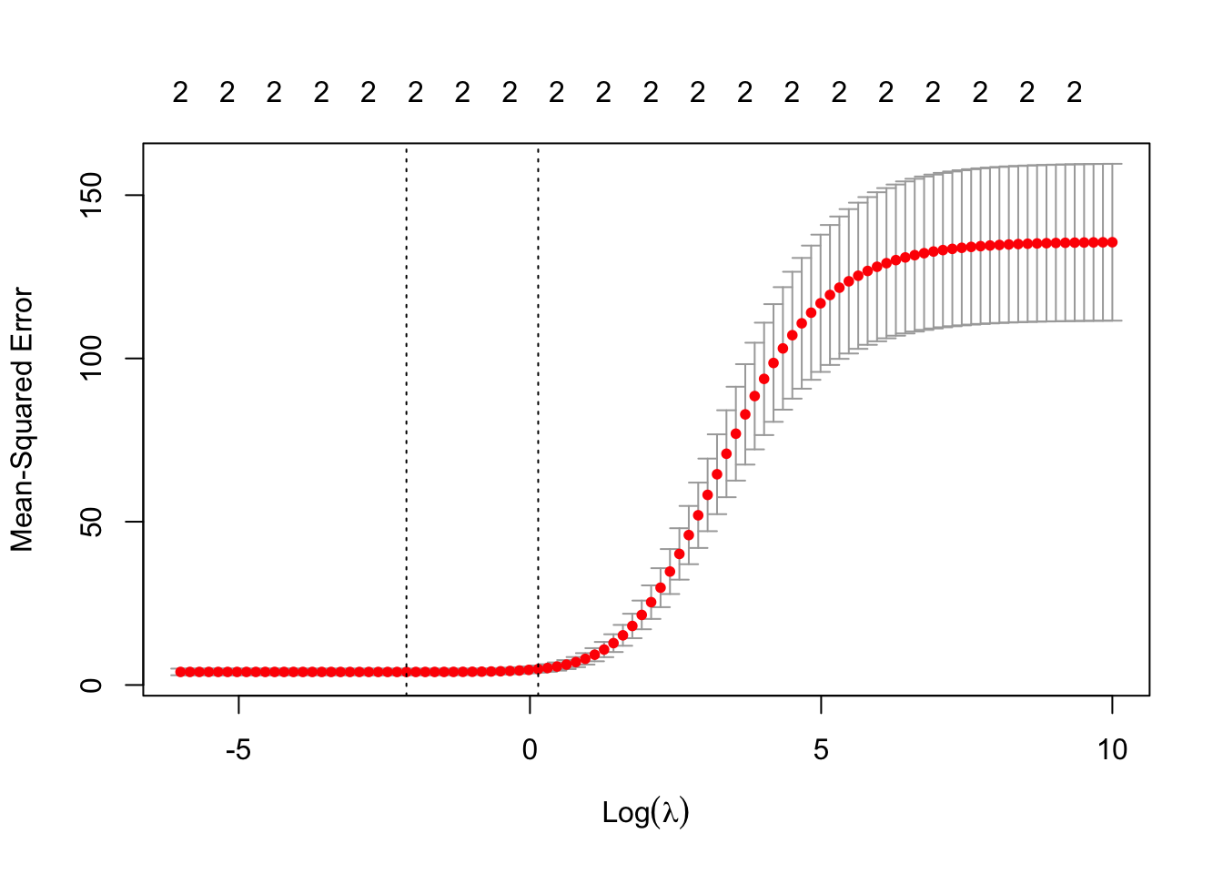
rrsim$lambda.min[1] 0.1198862Sure enough, the minimal predict error arises from a smaller \(\lambda\) than our original grid tested. We can now look at the actual model fits for the suggested values of lambda…
lammin <- rrsim$lambda.min
lam1se <- rrsim$lambda.1se
rrsimmin <- glmnet(x,y,alpha = 0, lambda=lammin)
rrsim1se <- glmnet(x,y,alpha = 0, lambda=lam1se)
coef(rrsimmin)
3 x 1 sparse Matrix of class "dgCMatrix"
s0
(Intercept) 19.458267
x1 3.050425
x2 -2.106344coef(rrsim1se)3 x 1 sparse Matrix of class "dgCMatrix"
s0
(Intercept) 19.581891
x1 2.811993
x2 -1.946284Lets throw those results into a table for easy comparison…
coeftab <- cbind(c(20.00,3.00,-2.00), coef(linmod), coef(rrsimmin), coef(rrsim1se))
colnames(coeftab) <- c("TRUE", "LM", "RidgeRegMin", "RidgeReg1se")
round(coeftab,2)
3 x 4 sparse Matrix of class "dgCMatrix"
TRUE LM RidgeRegMin RidgeReg1se
(Intercept) 20 19.44 19.46 19.58
x1 3 3.08 3.05 2.81
x2 -2 -2.13 -2.11 -1.95So ridge regression with the \(\lambda\) with estimated minimum MSE from CV provides estimates closer to the true values than the standard linear model approach as well as the ridge regression with \(\lambda\) within 1 standard error of the minimum. We can also run lasso using the glmnet command, the only difference is setting \(\alpha=1\) instead of 0…
lasim <- cv.glmnet(x, y, alpha=1, lambda=grid)
plot(lasim$glmnet.fit, label=TRUE, xvar="lambda")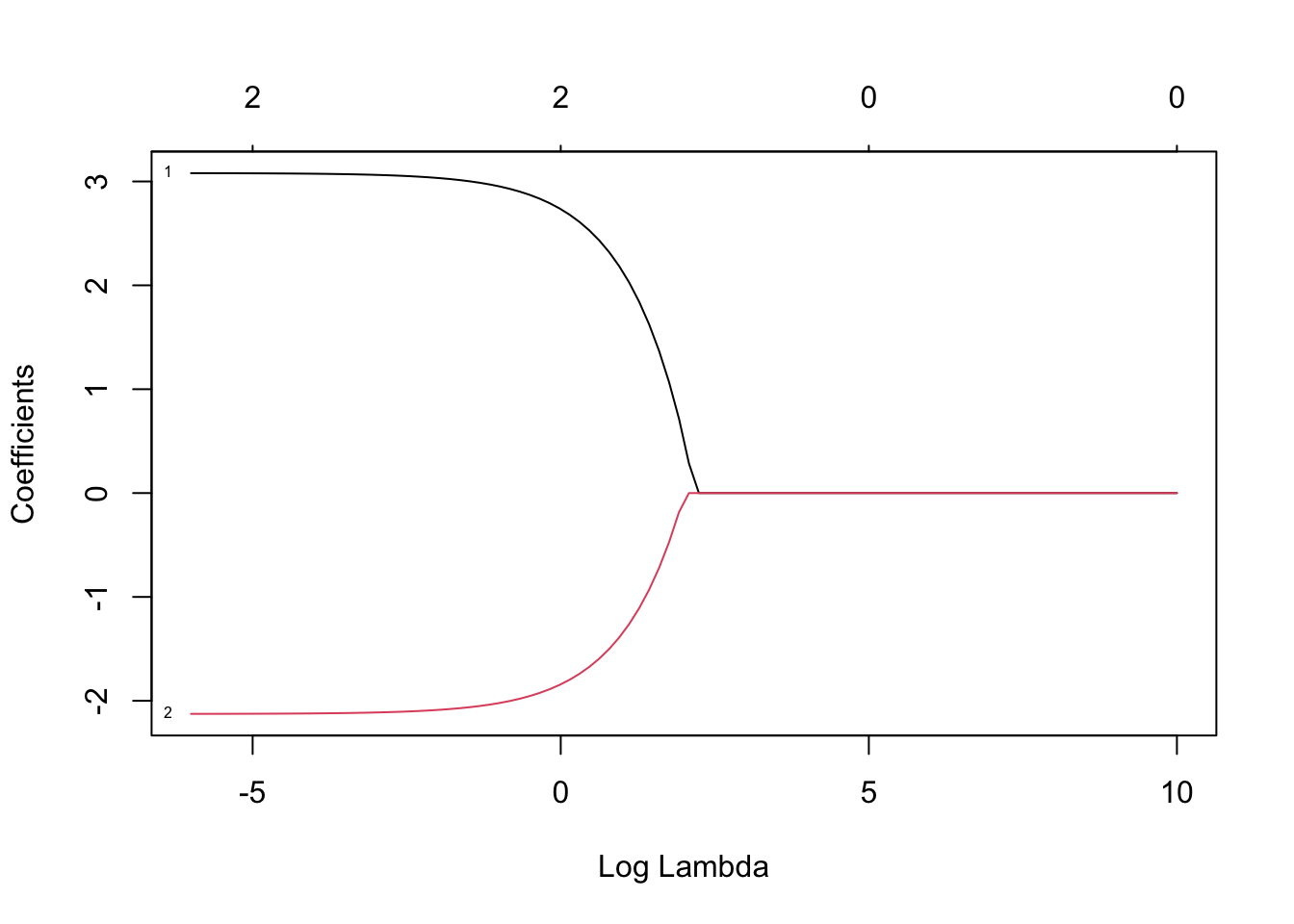
plot(lasim)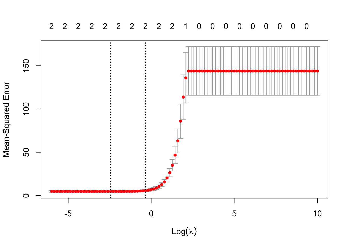
lammin <- lasim$lambda.min
lam1se <- lasim$lambda.1se
lasimmin <- glmnet(x,y,alpha = 1, lambda=lammin)
lasim1se <- glmnet(x,y,alpha = 1, lambda=lam1se)
coef(lasimmin)
3 x 1 sparse Matrix of class "dgCMatrix"
s0
(Intercept) 19.457600
x1 3.050666
x2 -2.101920coef(lasim1se)3 x 1 sparse Matrix of class "dgCMatrix"
s0
(Intercept) 19.565775
x1 2.834640
x2 -1.924461coeftab <- cbind(c(20.00,3.00,-2.00), coef(linmod), coef(rrsimmin), coef(lasimmin))
colnames(coeftab) <- c("TRUE", "LM", "RidgeRegMin", "LassoMin")
round(coeftab,2)3 x 4 sparse Matrix of class "dgCMatrix"
TRUE LM RidgeRegMin LassoMin
(Intercept) 20 19.44 19.46 19.46
x1 3 3.08 3.05 3.05
x2 -2 -2.13 -2.11 -2.10Results are essentially the same between ridge regression and lasso on this simulation. This is because to approach the true model, we only need to very slightly shrink the original estimates. Furthermore, there are no useless predictors to remove in this case. Let’s change that…
Let’s set up a model similar to the other one in lecture (and on assignment 1). A bunch of independent and useless predictors!
set.seed(52141)
bmat <- matrix(rnorm(50000), nrow=100)
dim(bmat)
[1] 100 500y <- rnorm(100)
bsimcv <- cv.glmnet(bmat, y, alpha=1)
plot(bsimcv)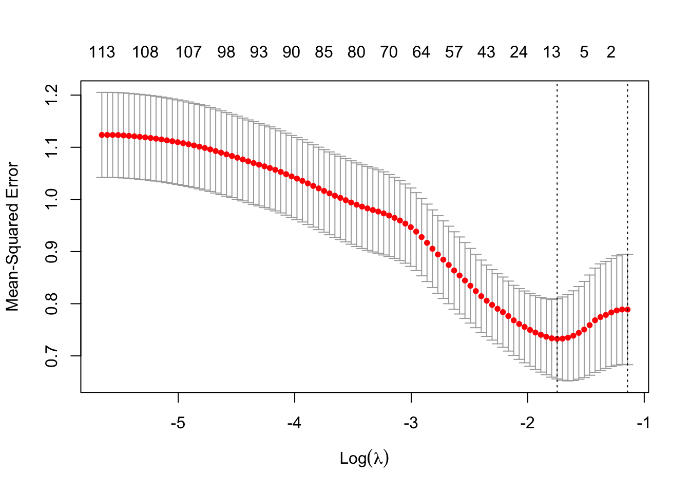
plot(bsimcv$glmnet.fit, label=TRUE, xvar="lambda")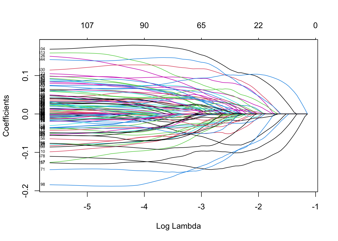
In this case, the lambda within 1 standard error appears to be at the boundary. So lets again manually specify a grid of lambda to see what happens…
grid <- exp(seq(-6, -1, length=100))
bsimcv2 <- cv.glmnet(bmat, y, alpha=1, lambda=grid)
plot(bsimcv2)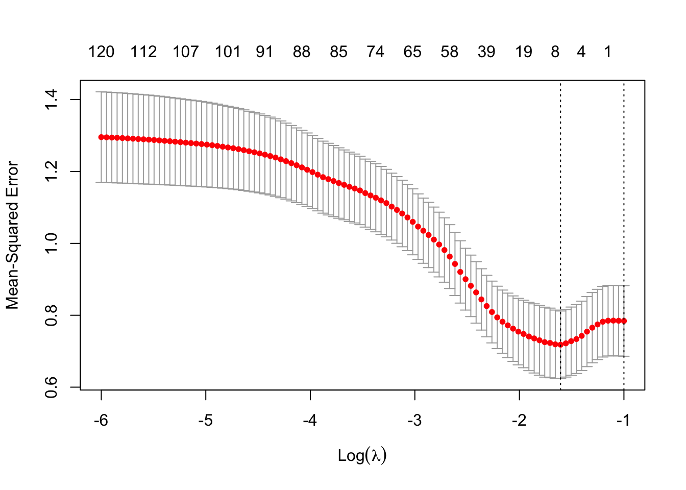
Interesting! The model that removes all predictors (and thereby only models according to the intercept) has a CV estimate of the MSE within 1 standard error of the minimum predicted MSE. This is a telltale sign that there are probably no useful predictors sitting in this data set!
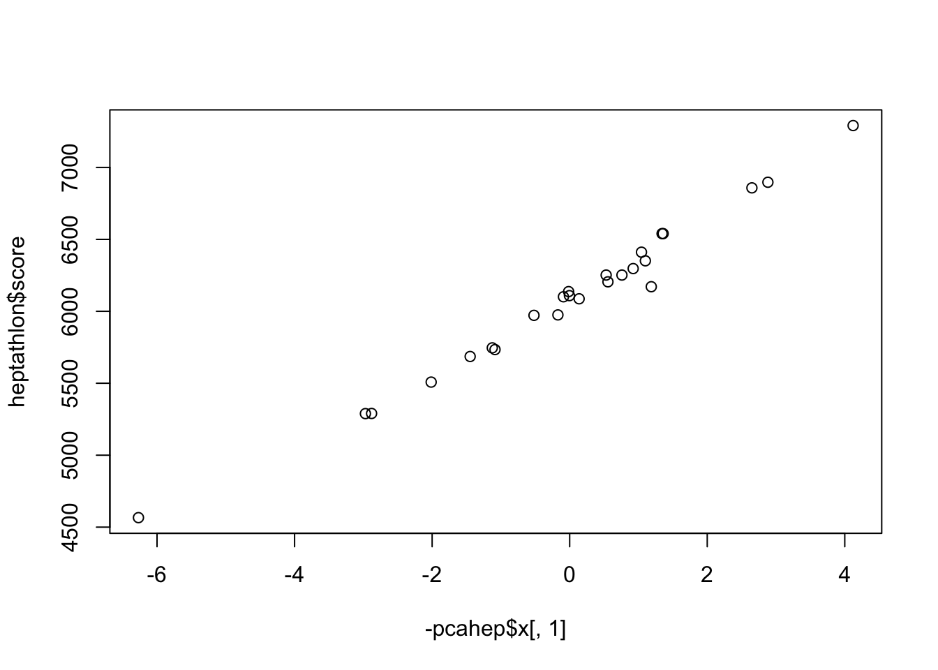
Principal Component Analysis (PCA) is a dimensionality reduction technique widely used in data analysis and machine learning. The main goal of PCA is to transform the original variables of a dataset into a new set of uncorrelated variables called principal components. These components are linear combinations of the original variables and are ordered by the amount of variance they capture.
library(HSAUR2) # to access the hepathalon dataLoading required package: toolsdata(heptathlon)library(HSAUR2)
data(heptathlon)
head(heptathlon) hurdles highjump shot run200m longjump javelin run800m
Joyner-Kersee (USA) 12.69 1.86 15.80 22.56 7.27 45.66 128.51
John (GDR) 12.85 1.80 16.23 23.65 6.71 42.56 126.12
Behmer (GDR) 13.20 1.83 14.20 23.10 6.68 44.54 124.20
Sablovskaite (URS) 13.61 1.80 15.23 23.92 6.25 42.78 132.24
Choubenkova (URS) 13.51 1.74 14.76 23.93 6.32 47.46 127.90
Schulz (GDR) 13.75 1.83 13.50 24.65 6.33 42.82 125.79
score
Joyner-Kersee (USA) 7291
John (GDR) 6897
Behmer (GDR) 6858
Sablovskaite (URS) 6540
Choubenkova (URS) 6540
Schulz (GDR) 6411pcahepu <- prcomp(heptathlon[,-8])
#Scree plot
plot(pcahepu, type="lines")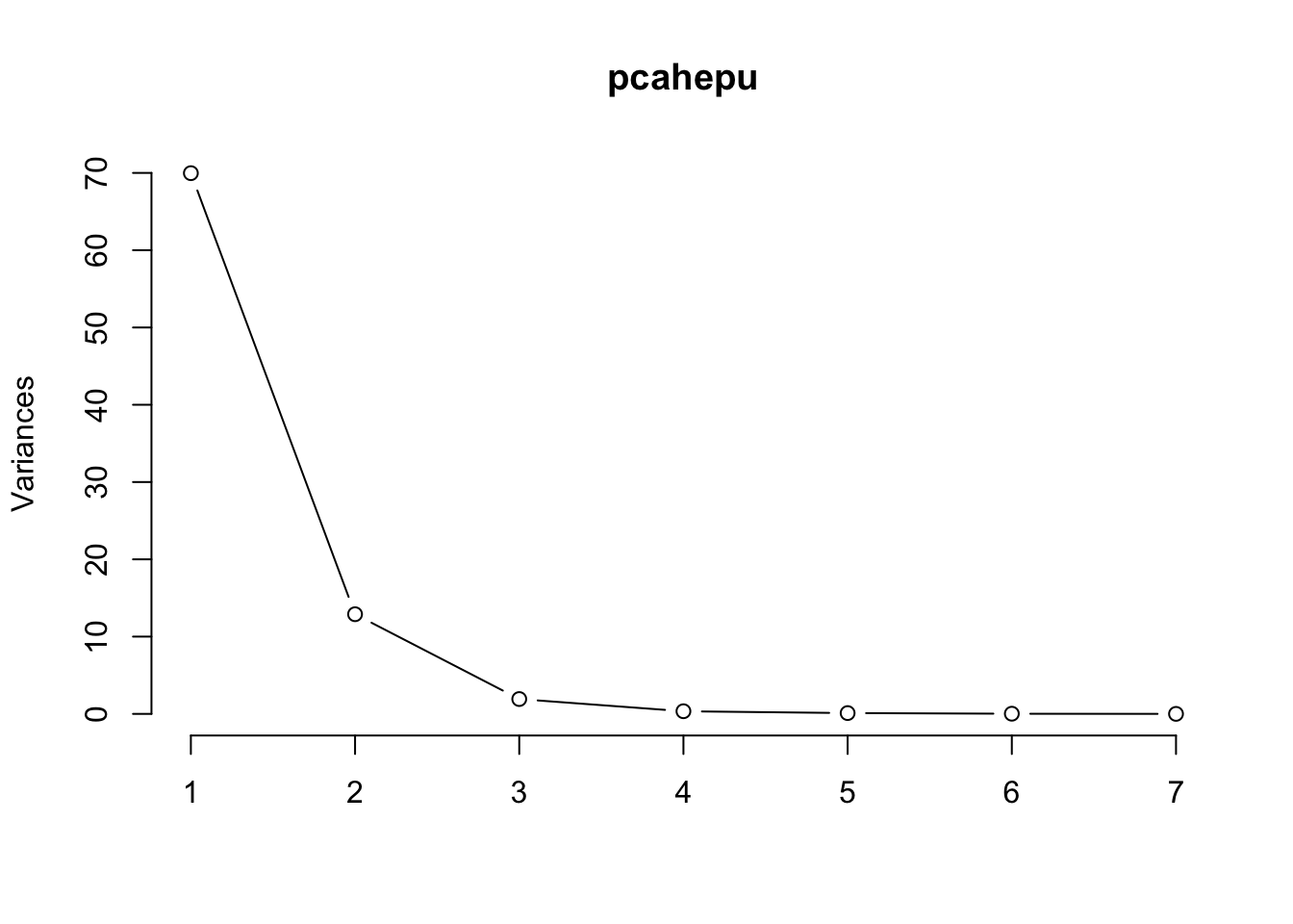
#Loadings, rotation matrix (eigenvectors) how the variables
#are correlated with each principal component
pcahepu$rotation[,1:3]
PC1 PC2 PC3
hurdles 0.069508692 0.0094891417 0.22180829
highjump -0.005569781 -0.0005647147 -0.01451405
shot -0.077906090 -0.1359282330 -0.88374045
run200m 0.072967545 0.1012004268 0.31005700
longjump -0.040369299 -0.0148845034 -0.18494319
javelin 0.006685584 -0.9852954510 0.16021268
run800m 0.990994208 -0.0127652701 -0.11655815round(pcahepu$rotation[,1:3], 2) PC1 PC2 PC3
hurdles 0.07 0.01 0.22
highjump -0.01 0.00 -0.01
shot -0.08 -0.14 -0.88
run200m 0.07 0.10 0.31
longjump -0.04 -0.01 -0.18
javelin 0.01 -0.99 0.16
run800m 0.99 -0.01 -0.12#Importance of components (variation explained)
summary(pcahepu)Importance of components:
PC1 PC2 PC3 PC4 PC5 PC6 PC7
Standard deviation 8.3646 3.5910 1.38570 0.58571 0.32382 0.14712 0.03325
Proportion of Variance 0.8207 0.1513 0.02252 0.00402 0.00123 0.00025 0.00001
Cumulative Proportion 0.8207 0.9720 0.99448 0.99850 0.99973 0.99999 1.00000pcahep <- prcomp(heptathlon[,-8], scale.=TRUE)
plot(pcahep, type="lines")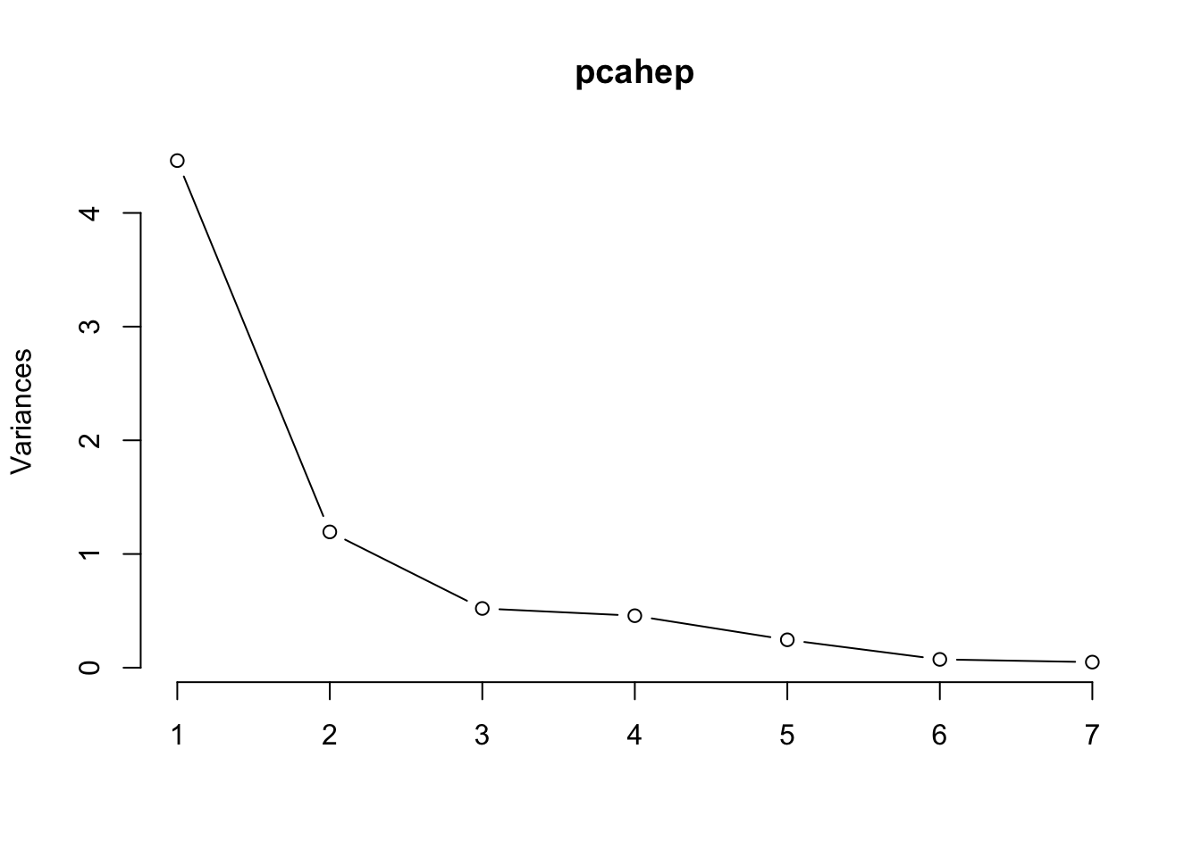
pcahep$rotation PC1 PC2 PC3 PC4 PC5 PC6
hurdles 0.4528710 -0.15792058 0.04514996 -0.02653873 -0.09494792 -0.78334101
highjump -0.3771992 0.24807386 -0.36777902 0.67999172 -0.01879888 -0.09939981
shot -0.3630725 -0.28940743 0.67618919 0.12431725 -0.51165201 0.05085983
run200m 0.4078950 0.26038545 -0.08359211 0.36106580 -0.64983404 0.02495639
longjump -0.4562318 0.05587394 0.13931653 0.11129249 0.18429810 -0.59020972
javelin -0.0754090 -0.84169212 -0.47156016 0.12079924 -0.13510669 0.02724076
run800m 0.3749594 -0.22448984 0.39585671 0.60341130 0.50432116 0.15555520
PC7
hurdles -0.38024707
highjump -0.43393114
shot -0.21762491
run200m 0.45338483
longjump 0.61206388
javelin 0.17294667
run800m 0.09830963round(pcahep$rotation[,1:3], 2) PC1 PC2 PC3
hurdles 0.45 -0.16 0.05
highjump -0.38 0.25 -0.37
shot -0.36 -0.29 0.68
run200m 0.41 0.26 -0.08
longjump -0.46 0.06 0.14
javelin -0.08 -0.84 -0.47
run800m 0.37 -0.22 0.40summary(pcahep)Importance of components:
PC1 PC2 PC3 PC4 PC5 PC6 PC7
Standard deviation 2.1119 1.0928 0.72181 0.67614 0.49524 0.27010 0.2214
Proportion of Variance 0.6372 0.1706 0.07443 0.06531 0.03504 0.01042 0.0070
Cumulative Proportion 0.6372 0.8078 0.88223 0.94754 0.98258 0.99300 1.0000biplot(pcahep)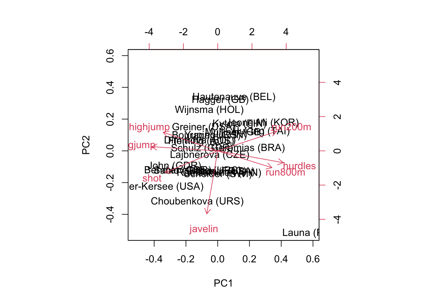
pcahep$x PC1 PC2 PC3 PC4
Joyner-Kersee (USA) -4.121447626 -1.24240435 0.36991309 0.02300174
John (GDR) -2.882185935 -0.52372600 0.89741472 -0.47545176
Behmer (GDR) -2.649633766 -0.67876243 -0.45917668 -0.67962860
Sablovskaite (URS) -1.343351210 -0.69228324 0.59527044 -0.14067052
Choubenkova (URS) -1.359025696 -1.75316563 -0.15070126 -0.83595001
Schulz (GDR) -1.043847471 0.07940725 -0.67453049 -0.20557253
Fleming (AUS) -1.100385639 0.32375304 -0.07343168 -0.48627848
Greiner (USA) -0.923173639 0.80681365 0.81241866 -0.03022915
Lajbnerova (CZE) -0.530250689 -0.14632191 0.16122744 0.61590242
Bouraga (URS) -0.759819024 0.52601568 0.18316881 -0.66756426
Wijnsma (HOL) -0.556268302 1.39628179 -0.13619463 0.40503603
Dimitrova (BUL) -1.186453832 0.35376586 -0.08201243 -0.48123479
Scheider (SWI) 0.015461226 -0.80644305 -1.96745373 0.73341733
Braun (FRG) 0.003774223 -0.71479785 -0.32496780 1.06604134
Ruotsalainen (FIN) 0.090747709 -0.76304501 -0.94571404 0.26883477
Yuping (CHN) -0.137225440 0.53724054 1.06529469 1.63144151
Hagger (GB) 0.171128651 1.74319472 0.58701048 0.47103131
Brown (USA) 0.519252646 -0.72696476 -0.31302308 1.28942720
Mulliner (GB) 1.125481833 0.63479040 0.72530080 -0.57961844
Hautenauve (BEL) 1.085697646 1.84722368 0.01452749 -0.25561691
Kytola (FIN) 1.447055499 0.92446876 -0.64596313 -0.21493997
Geremias (BRA) 2.014029620 0.09304121 0.64802905 0.02454548
Hui-Ing (TAI) 2.880298635 0.66150588 -0.74936718 -1.11903480
Jeong-Mi (KOR) 2.970118607 0.95961101 -0.57118753 -0.11547402
Launa (PNG) 6.270021972 -2.83919926 1.03414797 -0.24141489
PC5 PC6 PC7
Joyner-Kersee (USA) 0.42600624 -0.339329222 0.347921325
John (GDR) -0.70306588 0.238087298 0.144015774
Behmer (GDR) 0.10552518 -0.239190707 -0.129647756
Sablovskaite (URS) -0.45392816 0.091805638 -0.486577968
Choubenkova (URS) -0.68719483 0.126303968 0.239482044
Schulz (GDR) -0.73793351 -0.355789386 -0.103414314
Fleming (AUS) 0.76299122 0.084844490 -0.142871612
Greiner (USA) -0.09086737 -0.151561253 0.034237928
Lajbnerova (CZE) -0.56851477 0.265359696 -0.249591589
Bouraga (URS) 1.02148109 0.396397714 -0.020405097
Wijnsma (HOL) -0.29221101 -0.344582964 -0.182701990
Dimitrova (BUL) 0.78103608 0.233718538 -0.070605615
Scheider (SWI) 0.02177427 -0.004249913 0.036155878
Braun (FRG) 0.18389959 0.272903729 0.044351160
Ruotsalainen (FIN) 0.18416945 0.141403697 0.135136482
Yuping (CHN) 0.21162048 -0.280043639 -0.171160984
Hagger (GB) 0.05781435 0.147155606 0.520000710
Brown (USA) 0.49779301 -0.071211150 -0.005529394
Mulliner (GB) 0.15611502 -0.427484048 0.081522940
Hautenauve (BEL) -0.19143514 -0.100087033 0.085430091
Kytola (FIN) -0.49993839 -0.072673266 -0.125585203
Geremias (BRA) -0.24445870 0.640572055 -0.215626046
Hui-Ing (TAI) 0.47418755 -0.180568513 -0.207364881
Jeong-Mi (KOR) -0.58055249 0.183940799 0.381783751
Launa (PNG) 0.16568672 -0.255722133 0.061044365print(cbind(-sort(pcahep$x[,1]), rownames(heptathlon), heptathlon$score)) [,1] [,2] [,3]
Joyner-Kersee (USA) "4.12144762636023" "Joyner-Kersee (USA)" "7291"
John (GDR) "2.88218593484013" "John (GDR)" "6897"
Behmer (GDR) "2.64963376599126" "Behmer (GDR)" "6858"
Choubenkova (URS) "1.35902569554282" "Sablovskaite (URS)" "6540"
Sablovskaite (URS) "1.34335120967758" "Choubenkova (URS)" "6540"
Dimitrova (BUL) "1.18645383210095" "Schulz (GDR)" "6411"
Fleming (AUS) "1.10038563857154" "Fleming (AUS)" "6351"
Schulz (GDR) "1.0438474709217" "Greiner (USA)" "6297"
Greiner (USA) "0.923173638862052" "Lajbnerova (CZE)" "6252"
Bouraga (URS) "0.759819023916295" "Bouraga (URS)" "6252"
Wijnsma (HOL) "0.556268302151922" "Wijnsma (HOL)" "6205"
Lajbnerova (CZE) "0.53025068878324" "Dimitrova (BUL)" "6171"
Yuping (CHN) "0.137225439803273" "Scheider (SWI)" "6137"
Braun (FRG) "-0.0037742225569806" "Braun (FRG)" "6109"
Scheider (SWI) "-0.0154612264093339" "Ruotsalainen (FIN)" "6101"
Ruotsalainen (FIN) "-0.0907477089383117" "Yuping (CHN)" "6087"
Hagger (GB) "-0.171128651449235" "Hagger (GB)" "5975"
Brown (USA) "-0.519252645741107" "Brown (USA)" "5972"
Hautenauve (BEL) "-1.08569764619083" "Mulliner (GB)" "5746"
Mulliner (GB) "-1.12548183277136" "Hautenauve (BEL)" "5734"
Kytola (FIN) "-1.44705549915266" "Kytola (FIN)" "5686"
Geremias (BRA) "-2.01402962042439" "Geremias (BRA)" "5508"
Hui-Ing (TAI) "-2.88029863527855" "Hui-Ing (TAI)" "5290"
Jeong-Mi (KOR) "-2.97011860698208" "Jeong-Mi (KOR)" "5289"
Launa (PNG) "-6.27002197162808" "Launa (PNG)" "4566"plot(-pcahep$x[,1], heptathlon$score)