library(tree)
library(gclus) ## needed for the body data set
Loading required package: clusterdata(body)
btree <- tree(Gender~., data = body)Tree-based Methods
As it’s name suggests, Classification and Regression Trees (CART) can be used in the context of Classification or Regression. We will go over how to fit these trees in R and move to the more recent approach of random forests (introduced in the early 2000s). Random Forests, henceforth RF, uses bootstrapping to enhance these simple CART decision trees to be more competitive. Furthermore, RF will produce variance importance measures and leverage the so-called out-of-bag (OOB) observations to estimate error.
Tree-based methods for regression and classification involve segmenting the predictor space into a number of simple regions (hyper-rectangles) through recursive binary splitting. These splits correspond to internal nodes on a decision tree, i.e. a yes-no question related to a single predictor. By answering these series of questions for a given observation we navigate our way through the “branches” of the tree and end up at a terminal node, or “leaf”. All observations ending up in the same leaf will be predicted the same value. The predicted value is simply and average value (in the case of regression) or majority vote (in the case of classification) of the training observations that populate that hyper-rectangle in the predictor space.
Typically we “grow” these trees larger than we will need and “prune” them back by deleting some nodes. You will often hear me refer to these initial trees as “bushy trees”. We will be using the tree and randomForest packages for fitting, however, the ranger package for example, maybe be preferable to randomForest if you are working with high dimensional data as it is much faster.
bodyWe first use classification trees to analyze the body data set. The response Gender is a binary variable (1 - male, 0 - female). We can grow a tree with binary recursive partitioning using the remaining response variables using the following code:
library(tree)
library(gclus) ## needed for the body data setLoading required package: clusterdata(body)
btree <- tree(Gender~., data = body)To visualize the dendrogram we call the plot function on the resulting output (saved into R object btree). By default, the terminal nodes won’t be labelled. To add labels, call the text function on the tree objected:
plot(btree)
text(btree)
Hmmmm… does this look like you would have expected? Hint: look at the predictions at the terminal nodes. (Press the CODE button on the right to unhide the answer).
# We forgot to convert Gender to a factor!
# Hence tree() is thinking this is a regression
# rather than a classification problem
# To fix this we need to do:
body$Gender  = as.factor(body$Gender)
btree <- tree(Gender~., data = body)
plot(btree); text(btree)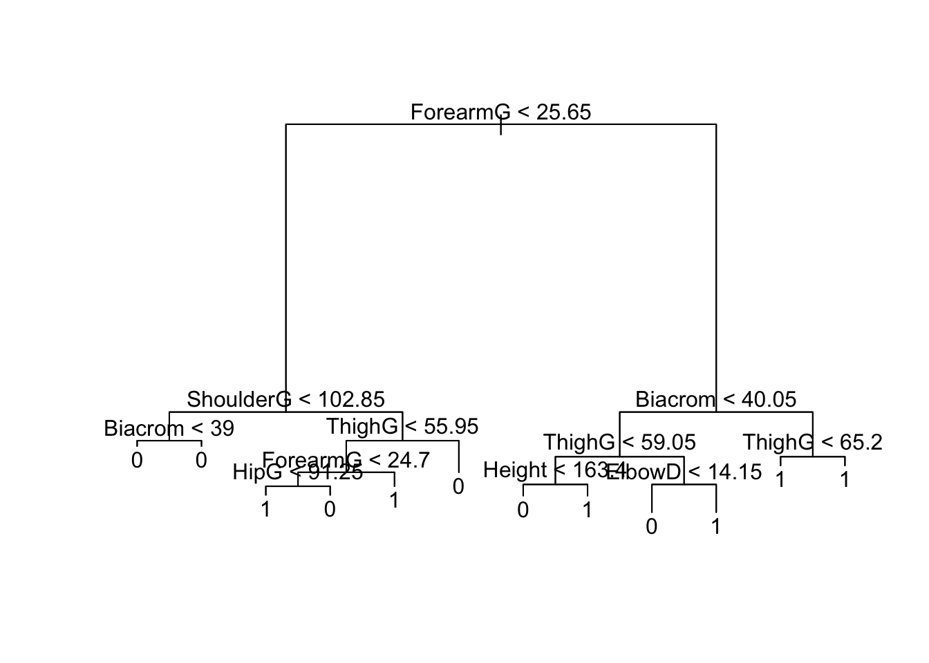
That looks better. To calculate the training error we use use:
tree.pred <- predict(btree, data = body, type="class")N.B if you try to run the above, you will get an error that ‘data’ must be a data.frame, environment, or list. The reason I think that this is happening is because tree() is confusing the body data frame with the function called body *see ?body1. To fix this, we’ll simply save our data set under a different name:
boddf = body
btree <- tree(Gender~., data = boddf)
tree.pred <- predict(btree, data = boddf, type="class")
(tree.tab <- table(boddf[,"Gender"], tree.pred,
                   dnn=c("True", "Predicted"))) # dim names
Predicted
True 0 1
0 256 4
1 3 244That is, we misclassified 7 of the 507 observations which is a misclassifaction rate of 1.4% computed using:
1 - sum(diag(tree.tab))/sum(tree.tab)[1] 0.01380671To check if we need to prune this tree back we use cross validation. Rather than coding it up ourselves we make use of the cv.tree function. By default it performs 10-fold cross validation.
set.seed(10) # set seed to make work reproducible
tree.cv <- cv.tree(btree)
plot(tree.cv, type="b")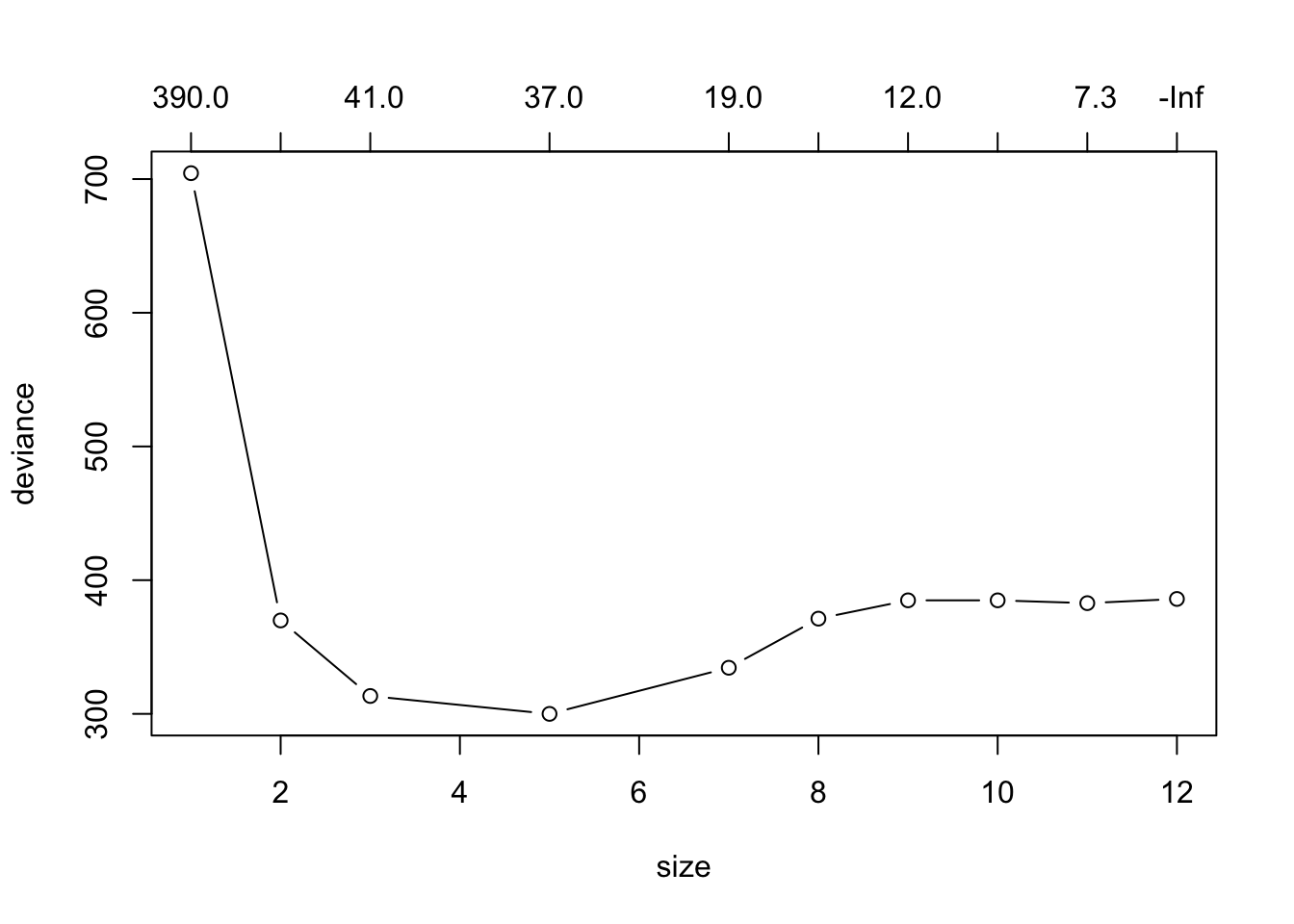
When plotting the results from cv.tree we look for which value the deviance (which in this case is the test misclassification error rate) is at it’s minimum. That will be our “best value” for the number of terminal nodes our bushy tree should be pruned back to have.
(best.val <- tree.cv$size[which.min(tree.cv$dev)])[1] 5We prune the tree using:
ptree <- prune.tree(btree, best=best.val)
plot(ptree); text(ptree)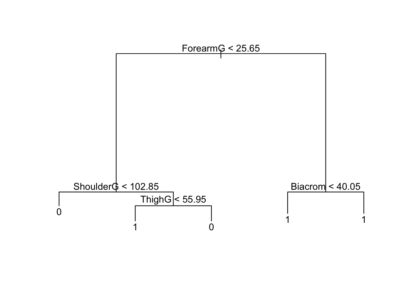
bodyLet’s perform bagging on the body data set using trees. Since there are 24 predictors in this set, we just tell R to perform random forests such that all predictors are considered at each split. This is done via the mtry command. Note that the importance=TRUE argument will allow us to make variable importance plots later.
library(randomForest)
set.seed(2331)
bodybag <- randomForest(Gender~., data=body, mtry=24, importance=TRUE)
bodybag
Call:
 randomForest(formula = Gender ~ ., data = body, mtry = 24, importance = TRUE)
               Type of random forest: classification
                     Number of trees: 500
No. of variables tried at each split: 24

        OOB estimate of  error rate: 5.13%
Confusion matrix:
    0   1 class.error
0 247  13  0.05000000
1  13 234  0.05263158
The misclassification rate quoted above is an out-of-bag OOB test error for the so-called “bagged” model. This misclassification rates, is based on the prediction obtained by the majority vote from trees that didn’t include that observation in the fitting process. As such, this estimate is comparable to estimates obtained from cross-validation.
We can also look at variable importance from the bagging model (if we omit importance=TRUE) from the randomForest call, only the MeanDecreaseGini plot will be shown.
varImpPlot(bodybag)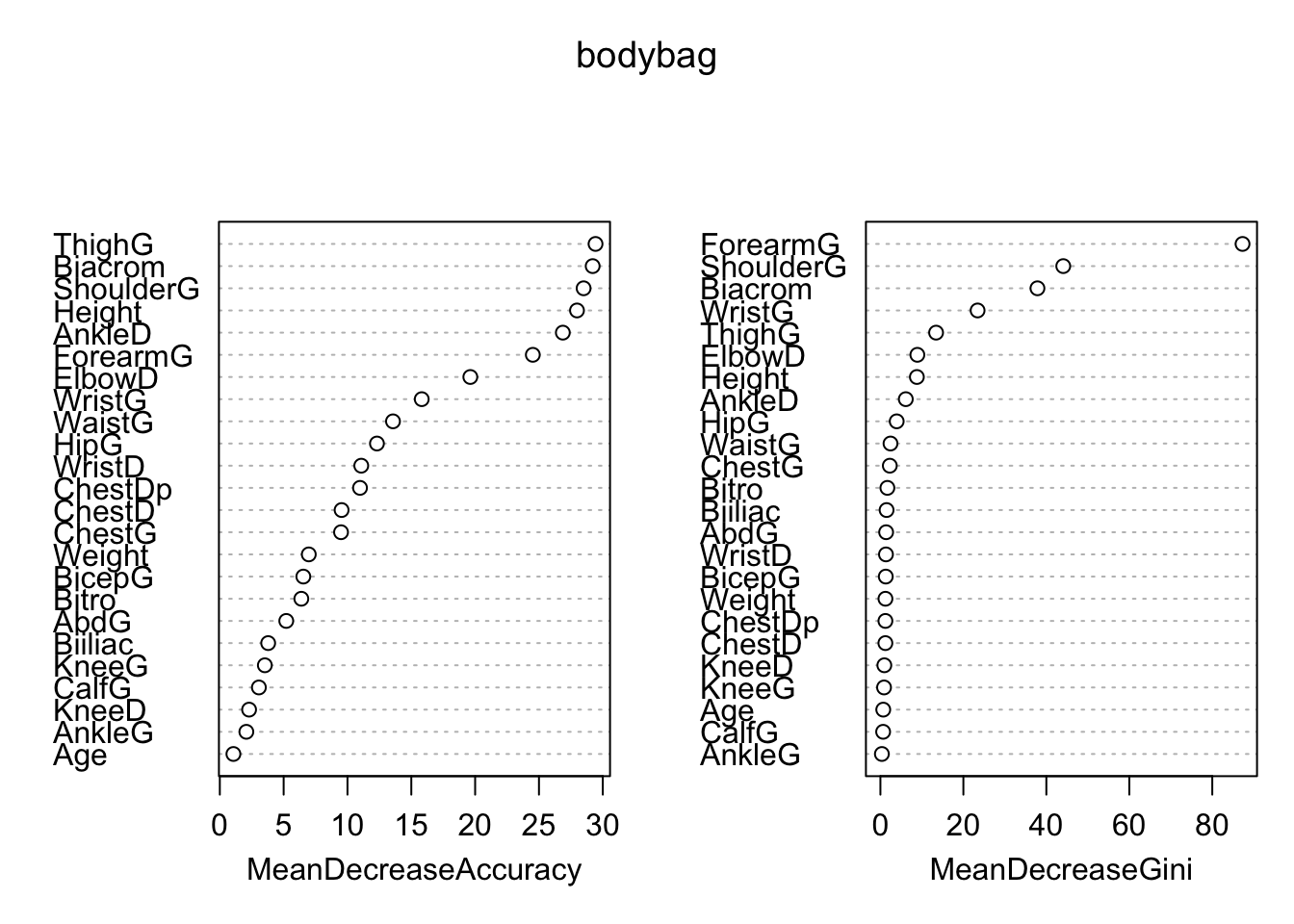
We can sse that actually numbers associated with the plot using:
importance(bodybag) 0 1 MeanDecreaseAccuracy MeanDecreaseGini
Biacrom 24.9064778 14.4492957 29.206567 37.8570069
Biiliac 2.4440142 3.0489251 3.787991 1.4888026
Bitro 5.8521617 3.6459842 6.385210 1.6818555
ChestDp 6.5053740 8.2019960 10.981341 1.2066011
ChestD -0.1751310 9.4650085 9.539489 1.2005494
ElbowD 15.6026802 11.5754258 19.623287 8.9073370
WristD 4.9139745 9.1894953 11.079683 1.3399518
KneeD 2.4129439 -0.0357201 2.292665 0.9464901
AnkleD 26.2256567 5.0649790 26.869681 6.1200468
ShoulderG 16.3022713 21.0077293 28.496664 44.0769107
ChestG 3.4693625 8.7656505 9.495298 2.2667095
WaistG 4.9529045 11.9633281 13.564975 2.4315843
AbdG 4.9346859 1.9129506 5.204297 1.3809284
HipG 11.6546812 7.4551773 12.308327 3.9269756
ThighG 27.6503589 18.3360110 29.431792 13.4232405
BicepG 3.0824846 5.0947449 6.541081 1.2957278
ForearmG 19.6011400 16.2305472 24.518063 87.2957535
KneeG 4.6410125 -1.2314965 3.526596 0.8759446
CalfG 3.4160937 0.8985015 3.060140 0.6566377
AnkleG 1.8385358 0.7464577 2.077605 0.3538577
WristG 11.9896447 9.3062421 15.816979 23.4268257
Age 0.6896869 0.8824248 1.064246 0.6860006
Weight 6.8671787 0.6451341 6.968465 1.2140868
Height 10.5023391 25.5209190 27.978446 8.7914260Recall that random forest grows \(B\)2 “bushy” trees and averages them. The only difference between bagging trees and random forests is that we randomly remove predictors from consideration at each binary split. This means our trees have (individually) less information to grow from…which leads to a larger variety of trees…and therefore less correlation across trees…and therefore more stability and better predictions (on average). See ?randomForest for mtry description…by default it is set to approx sqrt(p) for classification…
set.seed(4521)
bodyRF <- randomForest(Gender~., data=body, importance=TRUE)
bodyRF
Call:
 randomForest(formula = Gender ~ ., data = body, importance = TRUE)
               Type of random forest: classification
                     Number of trees: 500
No. of variables tried at each split: 4

        OOB estimate of  error rate: 3.94%
Confusion matrix:
    0   1 class.error
0 251   9  0.03461538
1 11 236 0.04453441varImpPlot(bodyRF)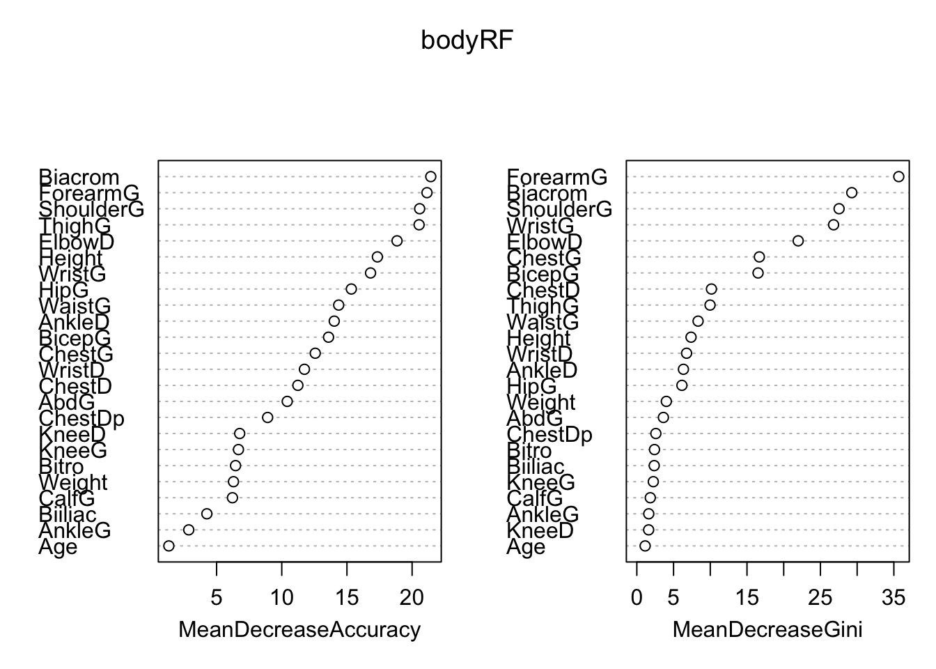
The above fits 500 trees (default value for ntree) and produce akin outputs to that shown for bagging.
I think it may be worthwhile revisiting one of the more difficult concepts in the course: that the 5-fold CV estimate of the MSE has less variance than the LOOCV estimate of the MSE.
To make the code easy, we’ll use regression trees since you can control the number of folds with the cv.tree function. We’ll need to simulate an example so that we can repeatedly generate new data — this is necessary in order to investigate the type of variance we’re discussing: how much a model (or estimate) changes when a new sample is taken.
set.seed(21341)
x <- runif(100, 0, 10)
y <- 5 + 2*x + rnorm(100)
plot(y~x)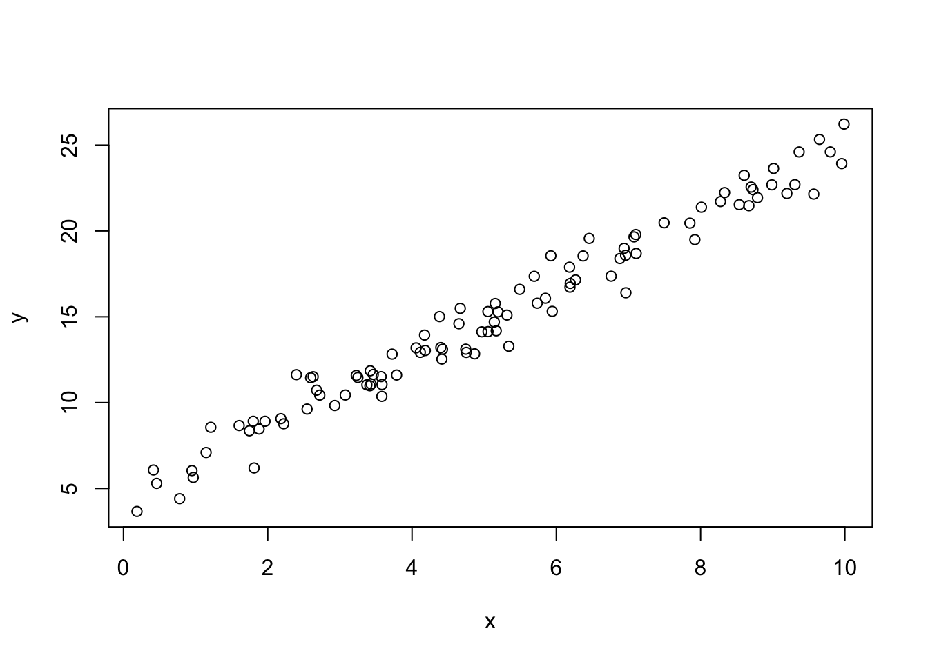
library(tree)
simtree <- tree(y~x)
loocv_simtree <- cv.tree(simtree, K=100)
loocv_RSS <- loocv_simtree$dev[1]
Since LOOCV is deterministic, we only need to compute it once for any data set. For the purposes of what we want to discuss though, 5-fold CV will have to be run several times (with the error saved). Off we go…
cv5_RSS <- NA
for(i in 1:500){
  cv5_simtree <- cv.tree(simtree, K=5)
  cv5_RSS[i] <- cv5_simtree$dev[1]
}
Now, we’ll give a histogram of the 5-fold estimates, and add the LOOCV estimate in red. BUT: THIS IS NOT ILLUSTRATING VARIANCE!!! WE ARE STILL ONLY LOOKING AT ONE DATA SET :)
hist(cv5_RSS)
abline(v=loocv_RSS, col="red")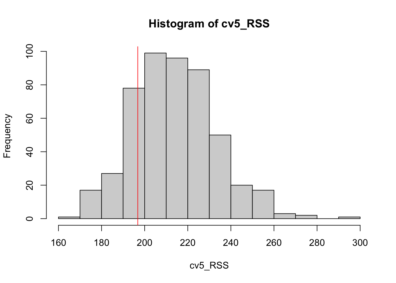
We don’t know the true MSE here for this nonparametric model fit to this type of data, but it’s worth noting that the center of the 5-fold estimates does appear above the LOOCV estimate (aka, more potential overestimation).
Now, let’s actually get to the variance part. We need to simulate a whole bunch of data, and we’ll fit both LOOCV and 5-fold-CV once each time…
set.seed(21)
loocv1k <- cv51k <- NA
for(i in 1:500){
  x <- runif(200, 0, 10)
  y <- 5 + 2*x + rnorm(200)
  simtree <- tree(y~x)
  loofit <- cv.tree(simtree, K=200)
  loocv1k[i] <- loofit$dev[1]
  cv5fit <- cv.tree(simtree, K=5)
  cv51k[i] <- cv5fit$dev[1]
}
Now, we will plot both separately, but on the same x-limits, for easier viewing…
par(mfrow=c(2,1))
xlims <- min(c(loocv1k, cv51k))-100
xlims[2] <- max(c(loocv1k, cv51k))+100
hist(loocv1k, xlim=xlims)
hist(cv51k, xlim=xlims)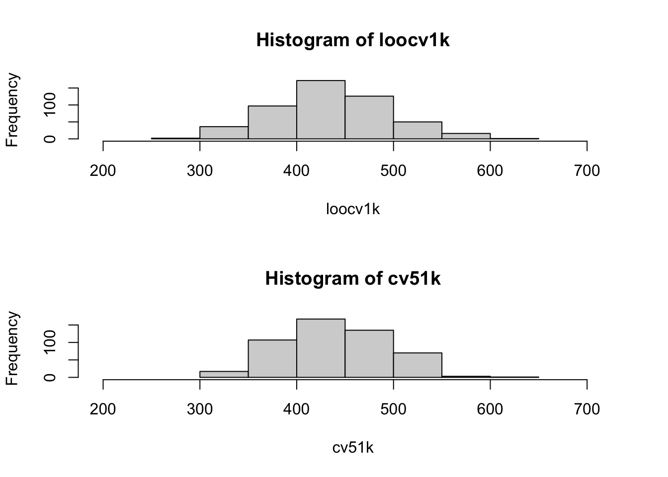
Or, obviously, literally compute the variance of the estimates…
var(loocv1k)[1] 3476.012var(cv51k)[1] 2738.313