Lab 7

Cross-validation and the Bootstrap

Author

Dr. Irene Vrbik

Published

October 1, 2023

Cross-validation

Cross validation is an alternative approach to training/testing split. For $k$ -fold cross validation, the dataset is divided into $k$ parts/folds. At iteration 1, the first fold is used as the testing set and the remaining $k - 1$ folds is used as the training set. The process is repeated $k$ times with each of the $k$ folds serving as the test set once. The out-of-sample performance, i.e. the performance metrics (e.g., accuracy, mean squared error, ROC-AUC) computed on each of the $k$ test sets, are averaged to produced the CV estimate.

LOOVC (manual)

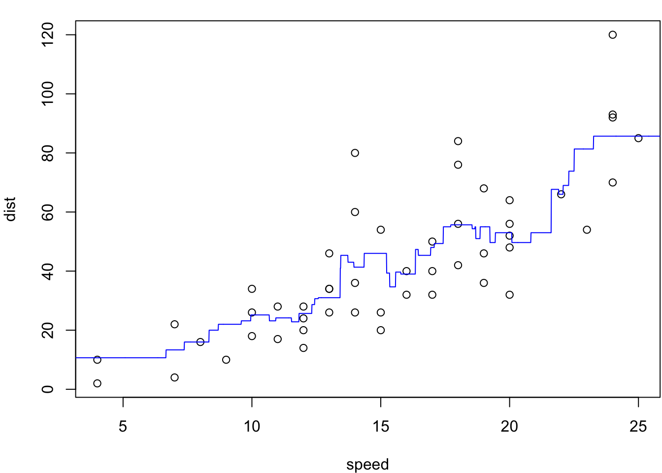
It’s relatively easy to set-up leave-one-out cross-validation yourself for any analysis. Here we can do it for the simple linear model…

data(cars)
attach(cars)
cvlm <- list()
msecv <- NA
for(i in 1:nrow(cars)){
  cvspeed <- speed[-i]
  cvdist <- dist[-i]
  cvlm[[i]] <- lm(cvdist ~ cvspeed)
  msecv[i] <- (predict(cvlm[[i]], newdata=data.frame(cvspeed=speed[i])) - dist[i])^2
}
mean(msecv)

[1] 246.4054

Which can be compared to unbiased estimate of the test MSE given $\hat{MSE} = \frac{RSS}{n - 2} = \frac{\sum (y_{i} - f (x_{i}))^{2}}{n - 2}$

lmfull <- lm(dist~speed)
sum(resid(lmfull)^2)/(nrow(cars) - 2)

[1] 236.5317

Notice that this estimate is larger than the training MSE (which we tend not to care to much about) given by the following:

mean((predict(lmfull)-dist)^2)

[1] 227.0704

k-fold (semi-manual)

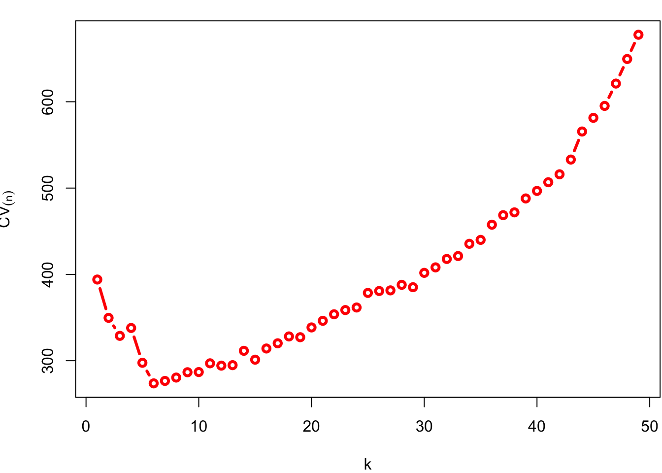
While it would be relatively easy to code up $k$ -fold CV validation ourselves, we can leverage the work of several packages to speed things up. For instance, in order to create $k$ folds we can use the createFolds() function from the caret package. For instance, if we instead wanted to do 6-fold cross validation:

library(caret)

Loading required package: ggplot2

Loading required package: lattice

k = 6 # number of folds

set.seed(123)  
folds <- createFolds(speed,       # a vector of outcomes
                     k = k)       # the number of folds required

mse_values <- numeric(k)          # a vector to store MSEi's

for (i in 1:k) {
  train_indices <- unlist(folds[-i])  # Training indices
  test_indices <- unlist(folds[i])    # Test indices

  # Fit the model on the training set
  model <- lm(dist ~ speed, data = cars[train_indices,])

  # Make predictions on the test set
  predictions <- predict(model, newdata = cars[test_indices,])

  # Calculate the Mean Squared Error (MSE)
  mse_values[i] <- mean((cars$dist[test_indices] - predictions)^2)
}

# Cross-Validated MSE estimate:
(cv_mse <- mean(mse_values))

[1] 238.5343

Using exisiting functions

Many analyses have CV built in. The boot package is a nice library which has handy functions and datasets for bootstrapping from the book Bootstrap Methods and Their Application by A. C. Davison and D. V. Hinkley (1997, CUP)

cv.glm

The cv.glm() function from the boot package calculates the estimated K-fold cross-validation prediction error for generalized linear models. Recall that these models have a shortcut formula so the model need only be fit once to obtain the CV estimates for MSE. To use the function we must first fit our regression model using glm():

lm.mod <- glm(dist~speed, data = cars) # default family is gaussian == lm()

Next we use the cv.glm() function to perform k-fold cross-validation:

set.seed(213456) 
library(boot)


Attaching package: 'boot'

The following object is masked from 'package:lattice':

    melanoma

cv_results <- cv.glm(data = cars, glmfit = lm.mod, K = k)

cv_results contains information about the cross-validation results. You can access various elements, including the mean squared error (MSE) for each fold.

names(cv_results)

[1] "call"  "K"     "delta" "seed"

cv_results contains information about the cross-validation results. More specifically the delta element is a vector whose first component is the raw cross-validation estimate. For regression problems you can access the cross-validation estimate for MSE using:

cv_results$delta[1]

[1] 235.3013

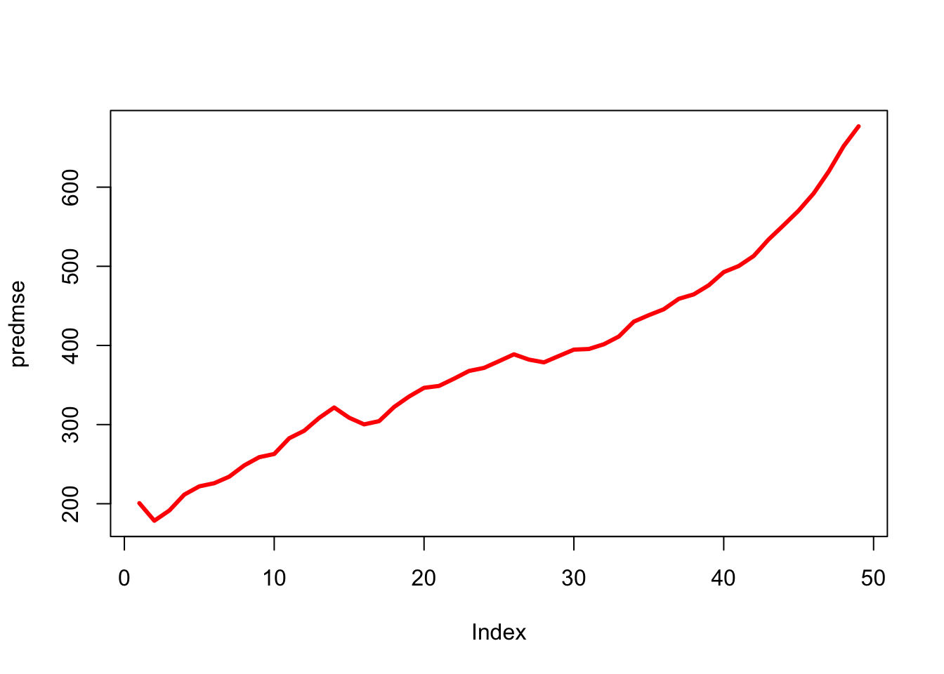
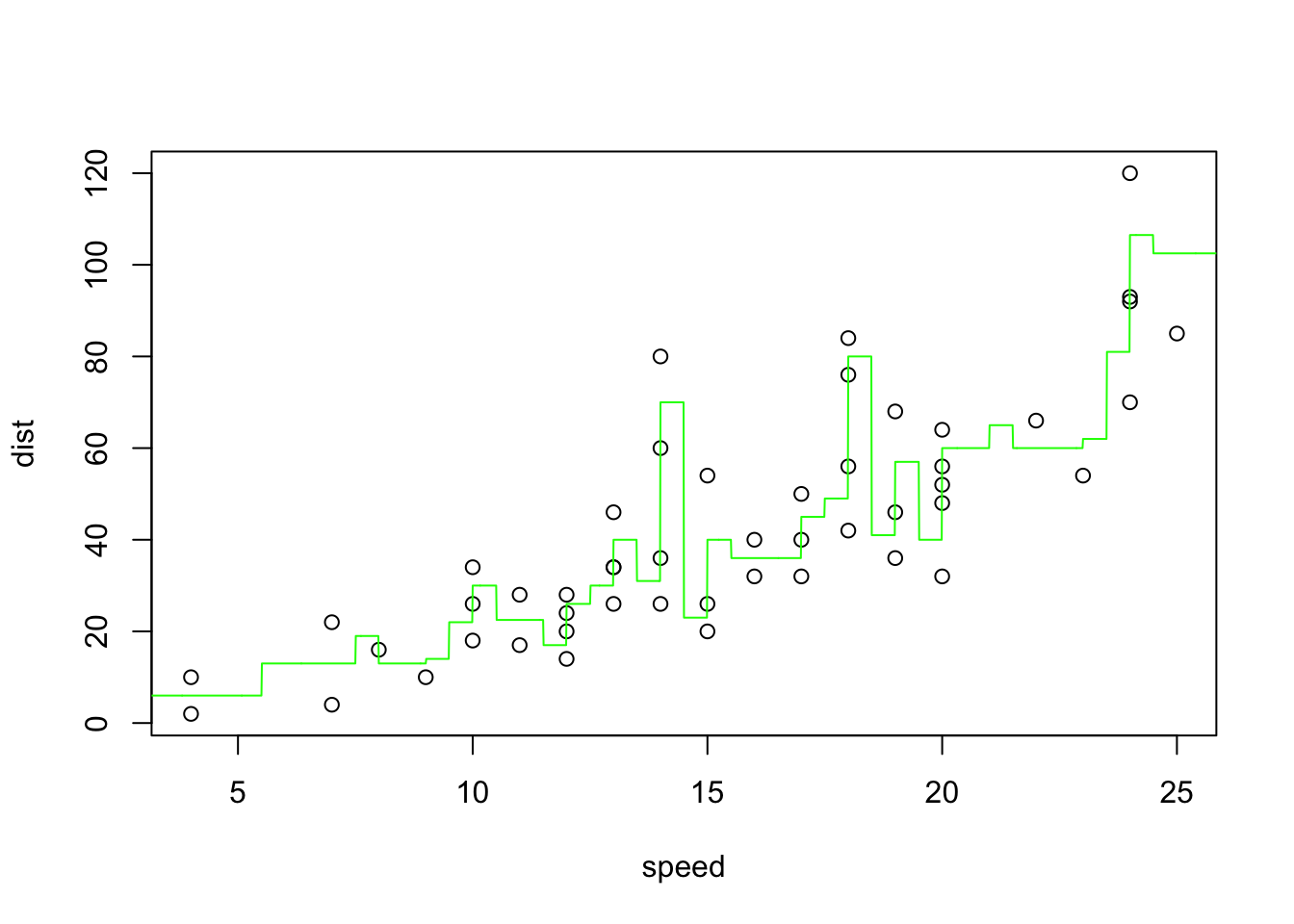
KNN regression

knn.reg() from the FNN package is another example of a function that has built-in (LOO) cross validation; see ?knn.reg. Here we can make use of that to choose the number of nearest neighbours for KNN regression.

library(FNN)
?knn.reg # note that knn.reg automatically uses CV in reporting
kr <- list()
predmse <- NA
for(i in 1:49){
  kr[[i]] <- knn.reg(speed, test=NULL, dist, k=i)
  predmse[i] <- kr[[i]]$PRESS/nrow(cars)
}
plot(predmse, type="l", lwd=3, col="red")

which.min(predmse)

[1] 2

plot(dist~speed)
seqx <- seq(from=0, to=30, by=0.01)
knnr <- knn.reg(speed, y=dist, test=matrix(seqx, ncol=1),  k=2) 
lines(seqx, knnr$pred, col="green", lwd=1)

As stated in lecture, these value does still appear to be overfitting to the data. This may be an artifact of how knn.reg deals with ties. Interestingly, we can see that if we “jitter” the data, i.e. add some random noise in the x-values, we get a different answer:

set.seed(93952)
speedj <- jitter(speed,4)
krj <- list()
predmsej <- NA
for(i in 1:49){
  krj[[i]] <- knn.reg(speedj, test=NULL, dist, k=i)
  predmsej[i] <- krj[[i]]$PRESS/nrow(cars)
}
par(mar = c(4, 4, 1.1, 0.1))
plot(predmsej, type="b", lwd=3, col="red", ylab = expression(CV[(n)]), xlab = expression(k))

(bestkj <- which.min(predmsej))

[1] 6

knn4 <- knn.reg(speedj, y=dist, test=matrix(seqx, ncol=1),  k=bestkj) 
plot(dist~speed)
lines(seqx, knn4$pred, col="blue", lwd=1)

Bootstrap

Manual

Here we will recreate the simulation provided in lecture for the nonparametric bootstrap

set.seed(311532)
x <- runif(30, 0, 1)
y <- 2*x + rnorm(30, sd=0.25)
mod1 <- lm(y~x)
newx <- list()
newy <- list()
modnew <- list()
coefs <- NA
for(i in 1:1000){
  #newx[[i]] <- runif(30, 0, 1)
  newx[[i]] <- x
  newy[[i]] <- 2*newx[[i]] + rnorm(30, sd=0.25)
  modnew[[i]] <- lm(newy[[i]]~newx[[i]])
  coefs[i] <- modnew[[i]]$coefficients[2]
}
set.seed(35134)
newboots <- list()
bootsmod <- list()
bootcoef <- NA
xy <- cbind(x,y)
for(i in 1:1000){
  newboots[[i]] <- xy[sample(1:30, 30, replace=TRUE),]
  bootsmod[[i]] <- lm(newboots[[i]][,2]~newboots[[i]][,1])
  bootcoef[i] <- bootsmod[[i]]$coefficient[2]
}

summary(mod1)$coefficients

               Estimate Std. Error     t value     Pr(>|t|)
(Intercept) -0.00427974 0.08754461 -0.04888639 9.613569e-01
x            2.05167004 0.12940570 15.85455727 1.620243e-15

sd(coefs)

[1] 0.1325126

sd(bootcoef)

[1] 0.132347

The theoretical standard error is 0.13735, so our hope is that all three values should be close to that. sd(coefs) (aside from the theoretical truth) would be a gold-standard approach for finding that value — but it is of course essentially impossible in practice to repeatedly gather new data. summary(mod1)$coefficients is based on the inferential linear regression assumptions (iid normal error, etc) and only one model fit. sd(bootcoef) is the bootstrap estimator based on resampling (with replacement) from the original sample.

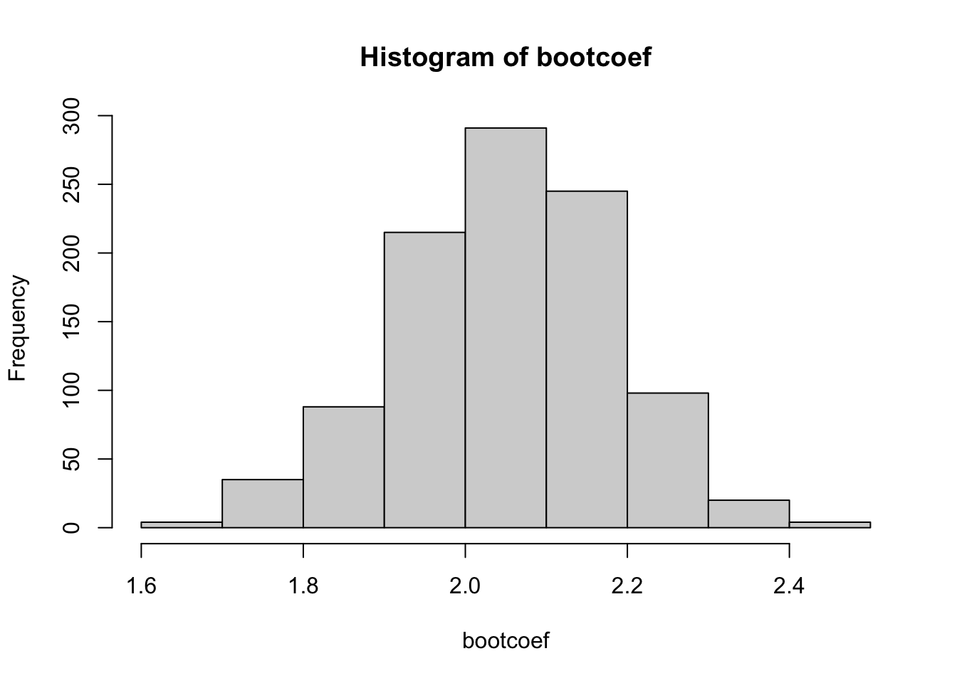
As in class, we can push further by using the observed bootstrap estimators in bootcoef as an empirical distribution. First, we looked at the histogram

hist(bootcoef)

The simplest bootstrap confidence interval, often called Efron intervals (after the bootstrap founder Bradley Efron), simply pull the relevant percentiles of the observed bootstrap estimates.

So for example, for an approx 95% CI we would want the 2.5th and 97.5th percentiles of the observed estimates…

quantile(bootcoef, c(0.025, 0.975))

    2.5%    97.5% 
1.766970 2.296553

How about a 90% CI? Well, that would need the 5th and 95th percentiles

quantile(bootcoef, c(0.05, 0.95))

      5%      95% 
1.825115 2.261882

Notice that the true theoretical value (2.00) is contained within both of these intervals.

Using exisiting functions

Alternatively we could use existing packages like boot to automate the bootstrapping process. These packages provide functions that simplify the implementation and often support parallel processing for efficiency.

For example we could redo the above example using:

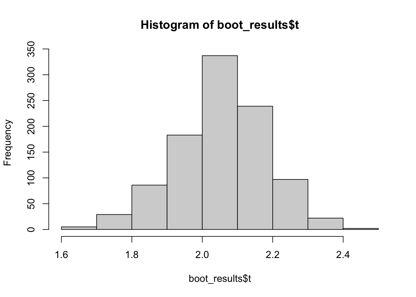
# Load the boot package
library(boot)

# Create a function to calculate the statistic of interest
beta_function <- function(data, indices) {
  sample_data <- data[indices,]
  fit <- lm(y~x, data = sample_data)
  return(coef(fit)["x"])
}

# Number of bootstrap samples
B <- 1000

# Set a seed for reproducibility
set.seed(6663492)

# Perform bootstrapping
dat <- data.frame(x, y)
boot_results <- boot(dat, beta_function, R = B)

# View the results
print(boot_results)


ORDINARY NONPARAMETRIC BOOTSTRAP


Call:
boot(data = dat, statistic = beta_function, R = B)


Bootstrap Statistics :
    original      bias    std. error
t1*  2.05167 0.002535141   0.1267117

Here beta_function() fits the linear regression model and pulls out the estimate for slope. More generally we will need to create a function that calculates our statistic (i.e. our function of our data, say, $T = t (X)$ ) out of resampled data. It should have at least two arguments: a data argument and an indices vector containing indices of elements from data that were picked to create a bootstrap sample.

boot_results have a few noteworthy outputs. $t contains the values our statistic $T (Z^{* j})$ where $Z^{* j}$ is the bootstrap sample and $j = 1, 2, \dots, B$ :

head(boot_results$t)

         [,1]
[1,] 2.093083
[2,] 2.070167
[3,] 1.914885
[4,] 1.917636
[5,] 1.936294
[6,] 2.078371

hist(boot_results$t)

$t0 contains values of our statistic(s) in original, full, dataset:

full.fit <- lm(y~x, data = dat)
coef(full.fit)["x"]

      x 
2.05167

boot_results$t0 # same as above

      x 
2.05167

The Bootstrap Statistics:

original is the same as $t0
bias is a difference between the mean of bootstrap realizations (averge of $t values), and the value in original dataset (saved to $t0).
std. error is a standard error of bootstrap estimate, which equals standard deviation of bootstrap realizations.

sd(boot_results$t) # std.error in Bootstrap Statitiscs

[1] 0.1267117