Lab 6

Clustering and cross-validation

Author

Dr. Irene Vrbik

Published

October 1, 2023

Clustering

Hierarchical Clustering

In this section we will fit the Hierarchical Clustering algorithm (HC) to some simulated data.

Single linkage chaining

Let’s simulate a weird data set with 2 clusters and a line of points running in between. We’ll use manhattan distance for no particular reason other than showing how to specify it…

library(MASS)
set.seed(3173)
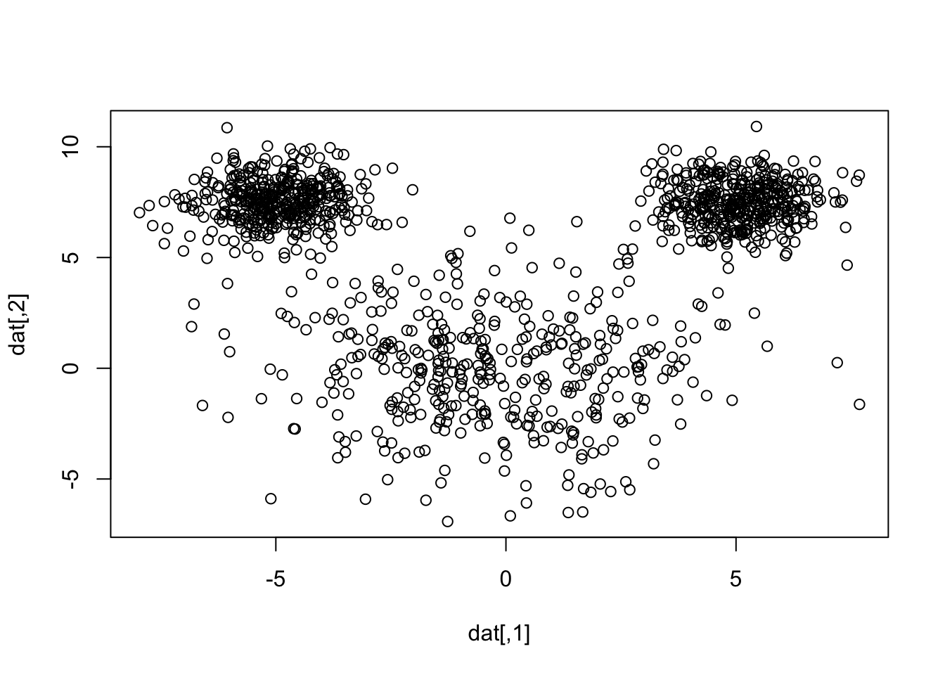
datagen1 <- mvrnorm(25, c(0,0), matrix(c(1,0,0,1),2,2))
datagen2 <- mvrnorm(25, c(5,-5), matrix(c(1,0,0,1),2,2))
datagen <- rbind(datagen1, datagen2)
x1 <- seq(from=0, to=5, by=0.2)
x2 <- seq(from=0, to=-5, by=-0.2)
newvalx <- cbind(x1,x2)
datagen <- rbind(datagen,newvalx)
plot(datagen)

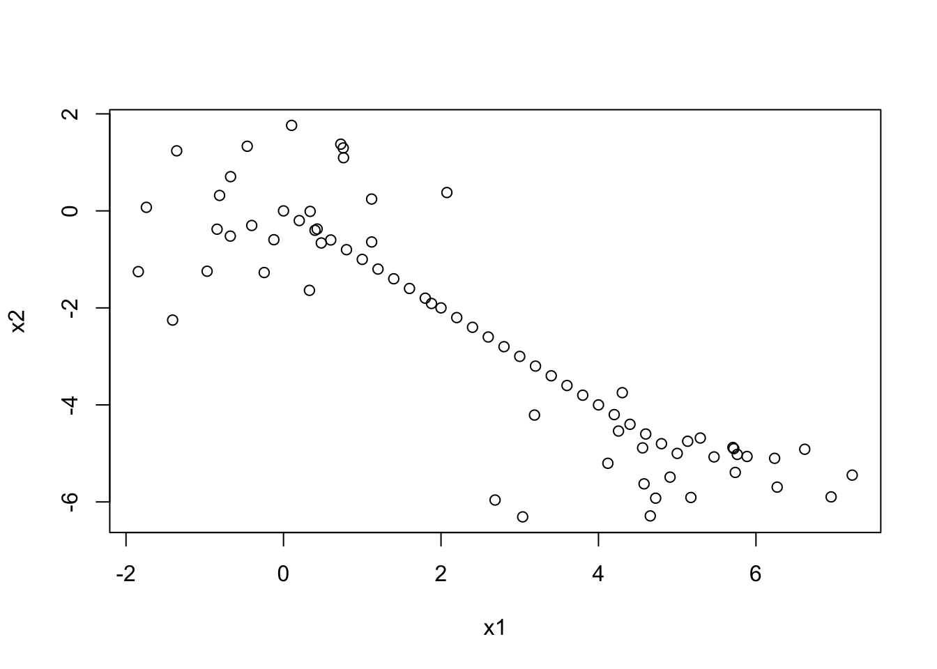
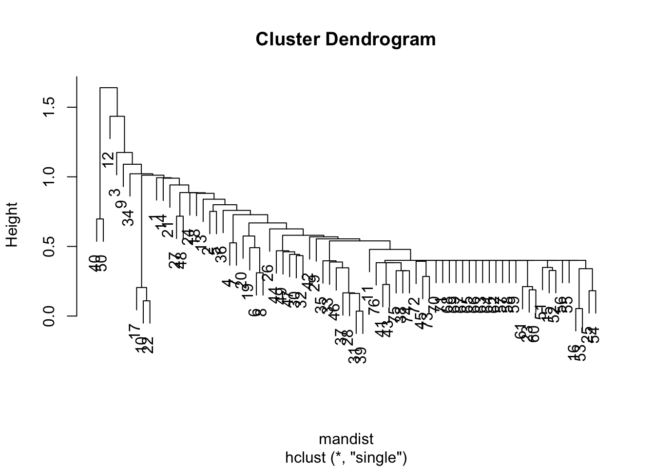
mandist <- dist(datagen,method="manhattan")
clus1 <- hclust(mandist, method="single")
plot(clus1)

Note that switching to euclidean distance doesn’t fix the issue, but does result in slightly different dendrogram:

eucdist <- dist(datagen,method="euclidean")
clus3 <- hclust(eucdist, method="single")
plot(clus3, main = "Single Linkaage")

The plots above is a tell-tale sign of the phenomena called “chaining” — essentially that you successively create one-member (i.e. singleton) clusters. This problem tends to only be a concern with single linkage since it only requires one pair of points close, irrespective of all others. Consequently for this data set, we will have major difficulty finding an underlying group structure using single linkage. If, however, we change the average linkage we get a much more better behaved dendrogram:

clus2 <- hclust(mandist, method="average")
plot(clus2, main = "Average Linkaage")

For the sake of completion, let’s observe the dendogram using the complete linkage method (which is the default)

clus4 <- hclust(mandist, method="complete")
plot(clus4, main = "Complete Linkaage")

Cutting the Tree

You can specify a height threshold in the dendrogram, and the tree is cut at that height. For instance we might cut the clus2 at a height of 6 and clust4 at 10.

mancom.h <- cutree(clus2, h = 6)
euccom.h <- cutree(clus4, h = 10)

Alternatively, you can specify the number of clusters you want, and the algorithm will cut the tree at a level that produces that number of clusters.

Here we specify where to cut the tree by requesting a specific number of groups, and then we can compare results between the average and complete-linkage two-group solutions:

mancom <- cutree(clus2,2) # same as mancom.h
euccom <- cutree(clus4,2) # same as euccom.h
table(mancom,euccom)
      euccom
mancom  1  2
     1 39  0
     2  0 37

Notice that these two methods produce the exact same paritioning of the data. Let’s visualize the clusters by colour on the scatterplot:

plot(datagen, col=mancom)

Now let’s compare the Euclidean with single linkage solution with the Euclidean with complete linkage solution.

eucsin <- cutree(clus3,2)
table(euccom, eucsin)
      eucsin
euccom  1  2
     1 39  0
     2 35  2

Single linkage makes two groups, one with only a single observation in it!

plot(datagen, col=eucsin)

Kmeans

Let’s code up k-means from scratch. We should be able to provide the function with the data x and the number of groups k.

It’s probably best to remind you of the steps of the kmeans algorithm first:

  1. Start with k random centroids (let’s use points within the data)
  2. Assign all observations to their closest centroid (by euclidean distance)
  3. Recalculate group means. Call these your new centroids.
  4. Repeat 2, 3 until nothing changes.

There are several ways of going about this. Sometimes its easier to just code the actual steps and then back up to setup the loop, etc, but I’ll provide the whole thing, with some comments to point out what we’re accomplishing with each chunk of the code.

my_k_means <- function(x, k){
  #1 start with k centroids
  centrs <- x[sample(1:nrow(x), k),]
  #start loop
  changing <- TRUE  
  while(changing){
    #2a) calculate distances between all x and centrs
    dists <- matrix(NA, nrow(x), k)
    #could write as a double loop, or could utilize other built in functions probably
    for(i in 1:nrow(x)){
      for(j in 1:k){
        dists[i, j] <- sqrt(sum((x[i,] - centrs[j,])^2)) 
      }
    }
    #2b) assign group memberships (you probably want to provide some overview of apply functions) 
    membs <- apply(dists, 1, which.min)
    
    #3) calculate new group centroids
    oldcentrs <- centrs #save for convergence check!
    for(j in 1:k){
      centrs[j,] <- colMeans(x[membs==j, ])
    }
    
    #4) check for convergence
    if(all(centrs==oldcentrs)){
      changing <- FALSE
    }
  }
  #output memberships
  membs
}

set.seed(5314)
#debug(my_k_means) #if you want
test <- my_k_means(scale(faithful), 2)
plot(faithful, col=test)

Compare to the built in version…

test2 <- kmeans(scale(faithful), 2)
plot(faithful, col=test2$cl)

Mouse simulation

kmeans

We’ll talk more about this near the end of the course, but here’s a very simple way to see some of the hidden assumptions of k-means in action.

library(mvtnorm)
set.seed(35151)
le <- rmvnorm(400, mean = c(-5,7.5))
re <- rmvnorm(400, mean = c(5,7.5))
hd <- rmvnorm(400, mean = c(0,0), sigma=7*diag(2) )
dat <- rbind(le, re, hd)
plot(dat)

mickres <- my_k_means(scale(dat), 3)
plot(dat, col=mickres)

table(mickres, rep(1:3, each = 400))
       
mickres   1   2   3
      1   0   0 361
      2 400   0  22
      3   0 400  17

After we do some class matching it looks like we are misclassifying 22 + 17 = 39 observations. Note how the smaller mouse ears are assumed larger in k-means, even though the groups are relatively well-separated. We can see this by showing a side by side of the truth and what k-means just gave us

par(mfrow=c(1,2))
plot(dat, col=mickres)
plot(dat, col=rep(c(2,3,1), each=400))

This is because k-means tries to find clusters that are of roughly equal size. It is imporant to understand this for problems in which your cluster sizes are quite different.

hclust

When we apply hierarchical clustering with complete linkage we get a more reasonable result, but still not perfect.

mickdist <- dist(scale(dat))
mickhc <- hclust(mickdist, method="complete")
mickhcres <- cutree(mickhc, 3)
plot(dat, col=mickhcres)

table(mickhcres, rep(1:3, each = 400))
         
mickhcres   1   2   3
        1 400   0  51
        2   0 400  16
        3   0   0 333

Try out some of the other linkage options on this data set to see if you can get one that performs better than the above

# average does a bit better
mickhc <- hclust(mickdist, method="average")
mickhcres <- cutree(mickhc, 3)
plot(dat, col=mickhcres)
table(mickhcres, rep(1:3, each = 400))