Lab 4

Logistic Regression and Classification Simulation

Author

Dr. Irene Vrbik

Published

October 1, 2023

So far we’ve assumed that our response variable was a quantitative value, i.e. the regression problem. In this lab we move to the classification setting wherein the response variable is categorical. While in lecture we usually referred to categories of $y$ as groups, or classes, to keep consistent with R terminology we will also be referring to the categorical variable as a factor variable, and it’s classes/groups as levels.

Data

The body dataset contains 21 body dimension measurements as well as age, weight (in kg), height (in cm), and gender (binary) on 507 individuals. You can find this in the gclus library as body. As always, lets load our data set into our R session and make sure that it looks as we expect.¹

library(gclus)
data(body)
attach(body)
head(body)

  Biacrom Biiliac Bitro ChestDp ChestD ElbowD WristD KneeD AnkleD ShoulderG
1    42.9    26.0  31.5    17.7   28.0   13.1   10.4  18.8   14.1     106.2
2    43.7    28.5  33.5    16.9   30.8   14.0   11.8  20.6   15.1     110.5
3    40.1    28.2  33.3    20.9   31.7   13.9   10.9  19.7   14.1     115.1
4    44.3    29.9  34.0    18.4   28.2   13.9   11.2  20.9   15.0     104.5
5    42.5    29.9  34.0    21.5   29.4   15.2   11.6  20.7   14.9     107.5
6    43.3    27.0  31.5    19.6   31.3   14.0   11.5  18.8   13.9     119.8
  ChestG WaistG AbdG HipG ThighG BicepG ForearmG KneeG CalfG AnkleG WristG Age
1   89.5   71.5 74.5 93.5   51.5   32.5     26.0  34.5  36.5   23.5   16.5  21
2   97.0   79.0 86.5 94.8   51.5   34.4     28.0  36.5  37.5   24.5   17.0  23
3   97.5   83.2 82.9 95.0   57.3   33.4     28.8  37.0  37.3   21.9   16.9  28
4   97.0   77.8 78.8 94.0   53.0   31.0     26.2  37.0  34.8   23.0   16.6  23
5   97.5   80.0 82.5 98.5   55.4   32.0     28.4  37.7  38.6   24.4   18.0  22
6   99.9   82.5 80.1 95.3   57.5   33.0     28.0  36.6  36.1   23.5   16.9  21
  Weight Height Gender
1   65.6  174.0      1
2   71.8  175.3      1
3   80.7  193.5      1
4   72.6  186.5      1
5   78.8  187.2      1
6   74.8  181.5      1

As you will notice in the print out above, Gender is being treated as a numeric integer (as indicated by <int> under the column heading) rather than a factor. If ever you are unsure if you are unsure if your variable is being treated as an integer or a factor, you can check using class

class(Gender)

[1] "integer"

As in the linear regression setting where we had to use something like lm(y~ x1 + factor(x2)) to let R know that a predictor variable is a categorical, we need to convert the Gender to the factor class to ensure that these values are being treated as a categories (i.e. levels) rather than numbers. To accomplish this we could run:

body$Gender <- factor(body$Gender)

Alternatively if we want to convert the 1’s to male and 0 to female² we could use something like:

body$Gender <- factor(body$Gender, levels = c(1,0), labels = c("male", "female"))

Now we can see that Gender is being treated as a categorical variable (i.e. a factor variable in R).

class(Gender)

[1] "integer"

Ooops! What have we forgot to do here?

Code

## Answer: we neglected to reattach the data set!
attach(body)

The following objects are masked from body (pos = 3):

    AbdG, Age, AnkleD, AnkleG, Biacrom, BicepG, Biiliac, Bitro, CalfG,
    ChestD, ChestDp, ChestG, ElbowD, ForearmG, Gender, Height, HipG,
    KneeD, KneeG, ShoulderG, ThighG, WaistG, Weight, WristD, WristG

While the data frame has changed it’s respective Gender column to a factor variable class(body$Gender) returns factor the object called Gender needs to be updated. To reattach, simple rerun the attach function³

Don’t be alarmed by the warning that reattaching your data set produces. It simply tells us that it’s overwriting the variables that were attached in the first version of body. Now we can see that Gender is being treated as a factor:

class(Gender)

[1] "factor"

Training and Testing

Before fitting our model, let’s divide our data into training and testing. To make our results reproducible let’s also set a seed⁴.

set.seed(1696623282) #  as.integer(Sys.time()) 
n <- nrow(body)
ptest <- 0.4 # 40% testing (60% training)
ntest <- round(n*ptest)
rind  = sample(n)
test_ind = rind[1:ntest]
train_ind = rind[(ntest+1):n]

test_data = body[test_ind, ]
train_data = body[train_ind, ]

Logistic Regression

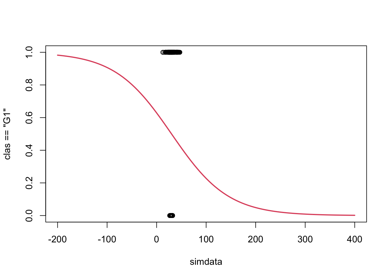
Now lets suppose we want to use Gender as the response variable. In that case we move from a Regression problem (with numeric continuous response) to a Classification problem (with discrete categorical response). We talked about in lecture why a regualar linear model is not sufficient. A possible alternative is logistic regression which is modeled by: $\log (\frac{P (Y = 1 ∣ X)}{1 - P (Y = 1 ∣ X)}) = β_{0} + β_{1} X_{1} + \dots + β_{p} X_{p}$

Logistic regression is a type of generalized linear models, hence we fit it using the glm function in R. In terms of inputs, it will feel very similar to using lm, i.e. its first input will be of the formula form Y~X. The family="binomial" indicates that R should fit logistic regression. Notice that since we already converted Gender to a factor we need not wrap the variable name in factor() in the lm function.

# simlog <- glm(factor(Gender) ~ Height , family="binomial")
simlog <- glm(Gender ~ Height , family="binomial",  subset = train_ind)
summary(simlog)


Call:
glm(formula = Gender ~ Height, family = "binomial", subset = train_ind)

Coefficients:
            Estimate Std. Error z value Pr(>|z|)    
(Intercept) 45.75626    5.13902   8.904   <2e-16 ***
Height      -0.26691    0.02999  -8.899   <2e-16 ***
---
Signif. codes:  0 '***' 0.001 '**' 0.01 '*' 0.05 '.' 0.1 ' ' 1

(Dispersion parameter for binomial family taken to be 1)

    Null deviance: 421.10  on 303  degrees of freedom
Residual deviance: 240.86  on 302  degrees of freedom
AIC: 244.86

Number of Fisher Scoring iterations: 5

Notice that the subset argument above allows us to specify the index of training observations in our full data set (as opposed to feeding the data frame of training observations). In other words, simlog is the equivalent to:

# same as
simlog2 <-  glm(Gender ~ Height , family="binomial", data = body, subset = train_ind)
simlog2


Call:  glm(formula = Gender ~ Height, family = "binomial", data = body, 
    subset = train_ind)

Coefficients:
(Intercept)       Height  
    45.7563      -0.2669  

Degrees of Freedom: 303 Total (i.e. Null);  302 Residual
Null Deviance:      421.1 
Residual Deviance: 240.9    AIC: 244.9

Something I unexpectedly discovered is that simlog and simlog2 is not the same as”

# not same as
simlog3 <-  glm(Gender ~ Height , family="binomial", data = train_data)
simlog3


Call:  glm(formula = Gender ~ Height, family = "binomial", data = train_data)

Coefficients:
(Intercept)       Height  
    45.7563      -0.2669  

Degrees of Freedom: 303 Total (i.e. Null);  302 Residual
Null Deviance:      421.1 
Residual Deviance: 240.9    AIC: 244.9

Why is that?

Code

## Because of the ordering of observations? Come back to this!

Notice from the outputs that we no longer have things like $r$ -squared values and $F$ tests. We will be discussing other metrics in a section below.

Prediction

Like with lm, the output of glm provides the estimates of the parameters. The logistic regression coefficients give the change in the log odds of the given observation being female⁵ for every one unit increase in the predictor variable. For this model:

$\begin{aligned} \log (\frac{P (Y = female ∣ X)}{1 - P (Y = female ∣ X)}) & = 45.7562552 + - 0.2669134 (H e i g h t) \\ ⟹ P (Y = female ∣ X) & = \frac{e^{45.7562552 + - 0.2669134 (H e i g h t)}}{1 + e^{45.7562552 + - 0.2669134 (H e i g h t)}} \end{aligned}$

Hence with a height of, say, 174:

\begin{aligned} P (Y = female ∣ X = 174) & = \frac{e^{45.7562552 + - 0.2669134 (174)}}{1 + e^{45.7562552 + - 0.2669134 (174)}} \\ = 0.3347727 \end{aligned}

We could find this probability more readily using the predict() function. Please note that the predict function will NOT work until your data is stored in in a data frame having the column names as the variables used in training your logistic regression above; see ?predict.lm for details.

# WRONG ways to specify 'newdata'
predict(simlog, newdata = 174, type = "response") # will produce error

# RIGHT way:
predict(simlog, newdata = data.frame(Height = 174), type = "response")

Since we will be reusing this data, let’s save it to an object:

newdata1 <- data.frame(Height = 174)
predict(simlog, newdata = newdata1, type = "response")

        1 
0.3347727

When we specify type = "response", the function returns the prediction as a probability = $P (Y = 1 | X)$ . By default, the predict function will return the lod-odds prediction:

# log odds are predicted by default
(log.odds.x<- predict(simlog, newdata = newdata1))

         1 
-0.6866771

# to convert to odds
(odds = exp(log.odds.x))

        1 
0.5032455

# to covert odds to probability ... 
(prob = odds/(1 + odds)) # same as above!

        1 
0.3347727

To convert the above probability into a classification, simply map observations to whichever class for which it has the highest probability of belonging. In our case $Pr (Y = female ∣ X = 174) =$ 0.3347727 (which implies $Pr (Y = male)) =$ 1 - 0.3347727 = 0.6652273), so the observation is predicted to be male. Since our response is binary (1 = female, 0 = male), any observations with resulting probabilities greater that 0.5 predicted as female.

For instance, lets see how this model would classify the objects in our test set:

# pred.gender <- predict(simlog, newdata = data.frame(body$Height),  type = "response") > 0.5
# predict gender for training set (same as above)
pred.prob <- predict(simlog, newdata=test_data,  type = "response") 
pred.gender <- factor(pred.prob>0.5, levels= c(FALSE, TRUE), labels=c("male", "female"))
y = test_data$Gender
# see the first 10:
head(cbind(pred.gender, y))

    pred.gender y
20            1 1
228           2 1
334           2 2
205           1 1
503           1 2
42            2 1

Which factor level do the probabilities correspond to?

For the binomial families, the “ $1$ ” in the $Pr (Y = 1 ∣ X)$ corresponds to the second level of our factor. Notice the order of the levels in the following output:

levels(Gender)

[1] "male"   "female"

In our case, since female is the second level, we will be predicting $P (Y = female ∣ X)$ .

Sidenote: By default R will order levels alphabetically. Our levels are not in alphabetical order because we hard coded them in the Data section. You can read more here for a discussion on how do I know which factor level of my response is coded as 1 in logistic regression?

Classification Performance

As discussed in lecture and in previous labs, we can summarize and compare our predictions to the truth using a confusion matrix. It can be found quickly using the table() function:

tab <- table(test_data$Gender, pred.gender)
tab

        pred.gender
         male female
  male     82     18
  female   16     87

with misclassification rate given by: $\frac{total misclassified}{total no. observations} = \frac{18 + 16}{203} = 0.1674877$

Simulation setup

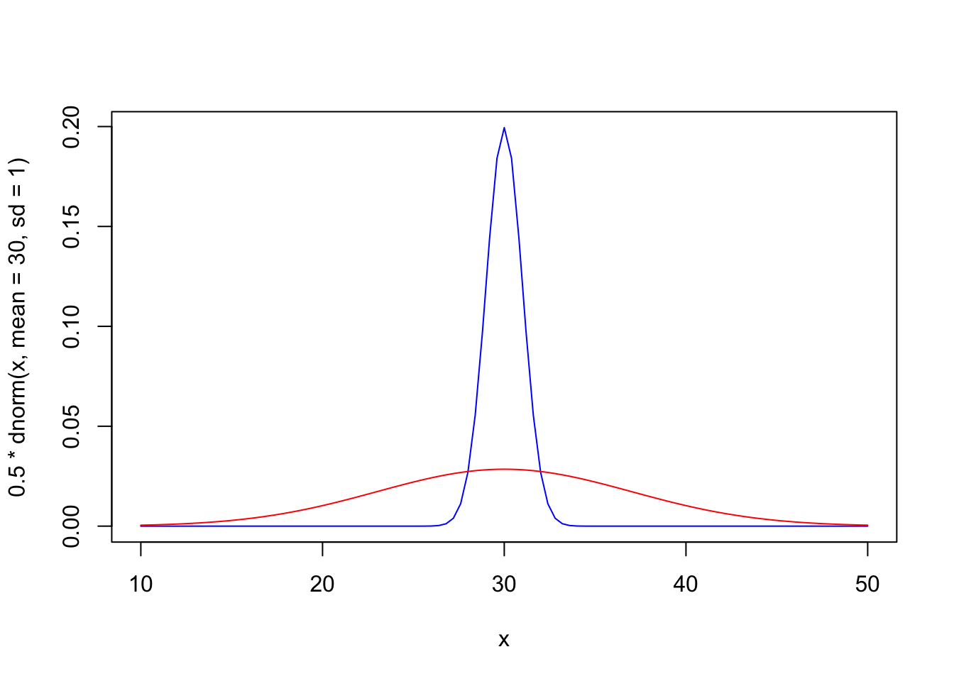
Let’s start off with a simulation that shows some insight beyond that discussed in lecture.

Suppose we have two groups, both normally distributed, with the same mean but different variance.

set.seed(3141)
g1 <- rnorm(200, mean=30, sd=7)
g2 <- rnorm(200, mean=30, sd=1)
#combine into one data set
simdata <- c(g1, g2)
#add group information
clas <- c(rep("G1", 200), rep("G2", 200))

This is a difficult classification problem, as the groups are essentially nested. Here’s the true generative distributions

curve(0.5*dnorm(x, mean=30, sd=1), from=10, to=50, col="blue",)
curve(0.5*dnorm(x, mean=30, sd=7), from=10, to=50, col="red", add=TRUE)

Now, let’s just use logistic regression to perform classification.

simlog <- glm(factor(clas) ~ simdata , family="binomial")
summary(simlog)


Call:
glm(formula = factor(clas) ~ simdata, family = "binomial")

Coefficients:
            Estimate Std. Error z value Pr(>|z|)
(Intercept)  0.52661    0.64329   0.819    0.413
simdata     -0.01749    0.02110  -0.829    0.407

(Dispersion parameter for binomial family taken to be 1)

    Null deviance: 554.52  on 399  degrees of freedom
Residual deviance: 553.83  on 398  degrees of freedom
AIC: 557.83

Number of Fisher Scoring iterations: 3

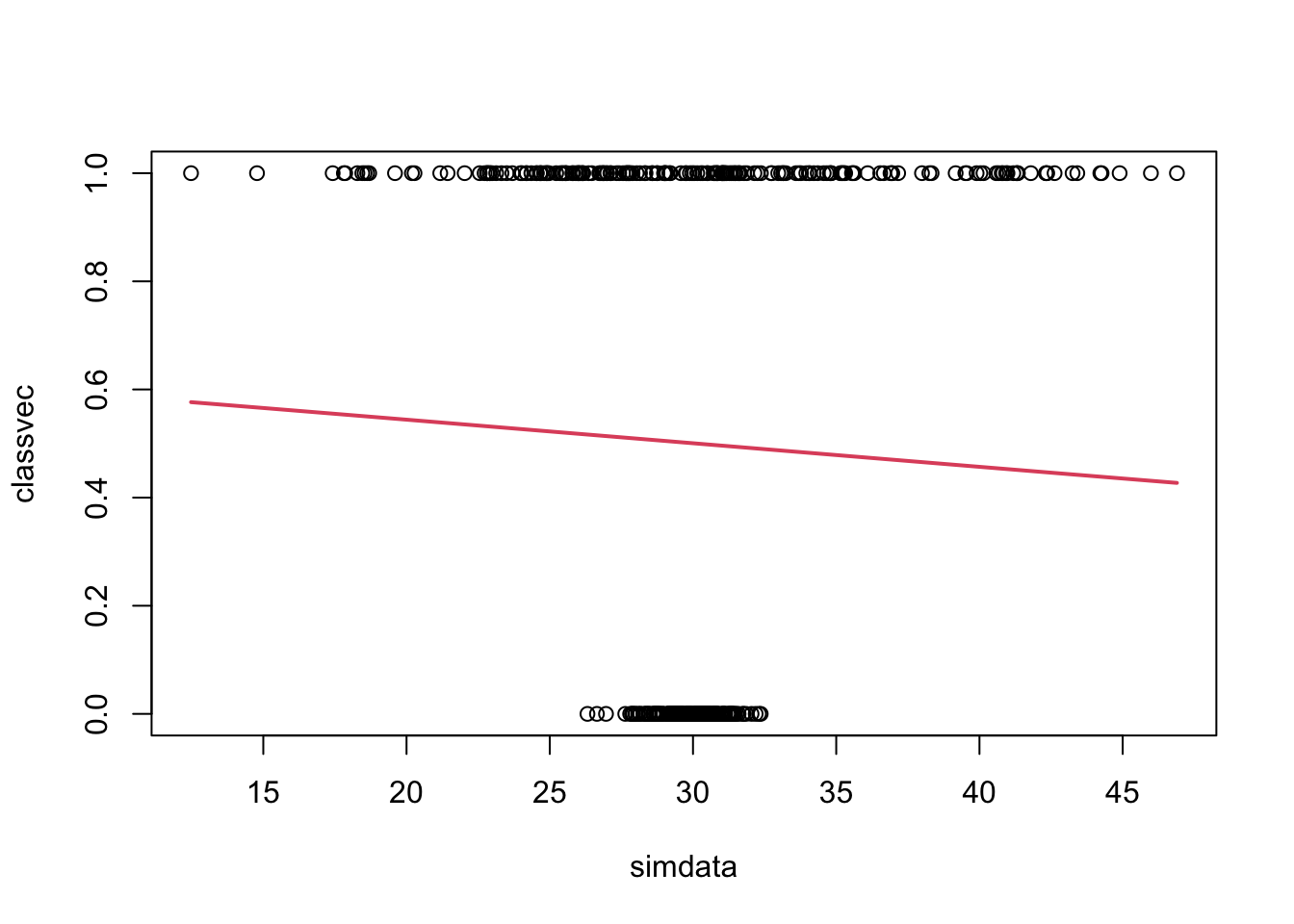
classvec <- clas == "G1" # 1 if group G1 0 o.w
plot(classvec ~ simdata)
betas <- coef(simlog);
curve((exp(betas[1] + betas[2]*x))/(1+exp(betas[1] + betas[2]*x)), add=TRUE, lwd=2, col=2)

# curve(exp(0.526-0.017*x)/(1+exp(0.526-0.017*x)), add=TRUE, col="blue", lwd=3)

In case you were wondering where the sigmoid function is, has a look at this zoomed out:

plot(clas == "G1" ~ simdata, xlim=c(-200,400))
betas <- coef(simlog);
curve((exp(betas[1] + betas[2]*x))/(1+exp(betas[1] + betas[2]*x)), add=TRUE, lwd=2, col=2)

To see our classification performance, let’s calculate the classification error rate:

(lr.tab = table(clas, predict(simlog, type="response") > .5))

    
clas FALSE TRUE
  G1    98  102
  G2    94  106

n = sum(lr.tab)
misclass = n - sum(diag(lr.tab))
err.rate = misclass/n

Terrible. A classification error rate of $\frac{196}{400}$ = 0.49. If we think about how we’re classifying, this result makes sense. Logistic regression assumes a single boundary, which isn’t appropriate in this context. Quadratic discriminant analysis is the correct model…

Quadratic Discriminant Analysis

To fit Quadratic Discriminant Analysis (QDA) we use the qda function from the MASS library.

library(MASS)
simqda <- qda(clas~simdata)
table(clas, predict(simqda)$class)

    
clas  G1  G2
  G1 149  51
  G2  11 189

Much better. Misclassification rate of 62/400 = 0.155.

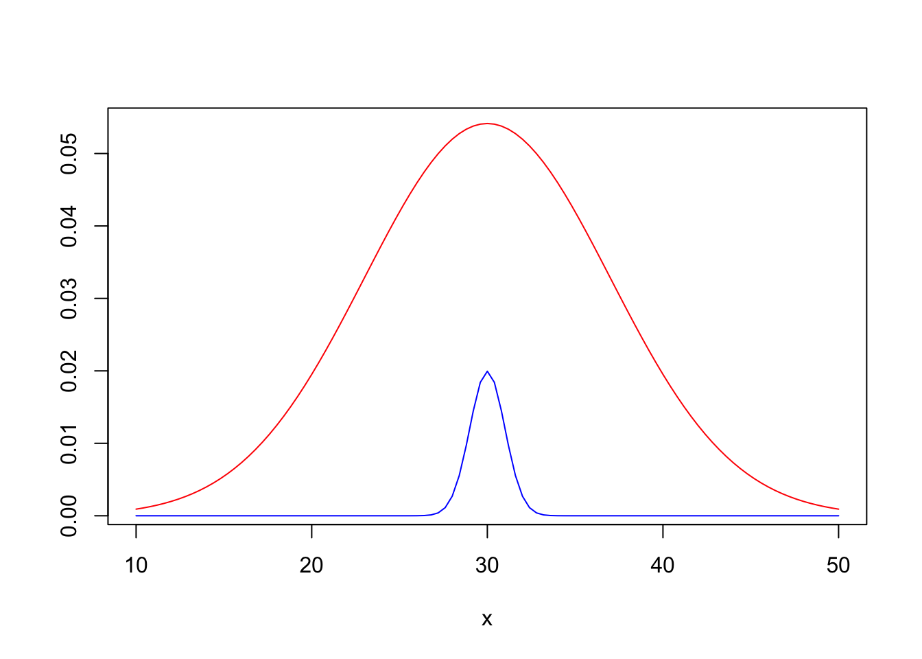
But what if one of the groups has fewer observed values? Let’s copy and paste some earlier commands and make adjustments. Make sample sizes of G1 380 and G2 20.

set.seed(3141)
g1 <- rnorm(380, mean=30, sd=7)
g2 <- rnorm(20, mean=30, sd=1)
simdata <- c(g1, g2)
clas <- c(rep("G1", 380), rep("G2", 20))
simlog <- glm(factor(clas) ~ simdata , family="binomial")
table(predict(simlog, type="response") > .5, clas)

       clas
         G1  G2
  FALSE 380  20

simqda <- qda(clas~simdata)
table(clas, predict(simqda)$class)

    
clas  G1  G2
  G1 380   0
  G2  20   0

So we technically have a ‘misclassification rate’ of 20/400 = 0.05…but in reality, this ‘low’ rate is equivalent to saying “I guess group 1, no matter what the data says”! In fact, we are misclassifying 100% of the G2 (blue) group. Hence, why we have discussed performance metrics in more detail.

But why is this case so much harder? Consider the proportions associated with each group (those $π_{g}$ discussed in lecture). In that case we have…

curve(380/400 * dnorm(x, mean=30, sd=7), from=10, to=50, col="red", ylab="")
curve(20/400 * dnorm(x, mean=30, sd=1), from=10, to=50, col="blue",  add=TRUE)

So no intersections! With the data we have, we will never be able to perform classification. That’s because the Bayes Classifier would even claim that everything is in the red group!

Comparing Classification Methods

Footnotes

For example, you can call View(...) or head(...) or srt(...) on your data set to accomplish this.↩︎
the information regarded this encoding can be found in the help file for the body data set which can be accessed using ?body↩︎
Ideally, you should do any adjustments to your data frame before you attach your data set.↩︎
In case you were wondering how a generate this seed, I used as.integer(Sys.time()). I like to do this to avoid using similar seeds over and over again, e.g. set.seed(<year>).↩︎
see this section for explanation of how we know which factor level is coded as 1↩︎