Data 311: Machine Learning

Lecture 20 - Deep Learning

Dr. Irene Vrbik

University of British Columbia Okanagan

Background

• Neural networks (NN) is a supervised machine learning algorithms that rose to fame in the late 1980s

• Automatic methods like Support Vector Machines (SVM), boosting, and random forests caused NN, which required a lot of tinkering, to take a backseat.

• Neural networks resurfaced after 2010 with the new name deep learning and by 2020 they are one of the most popular algorithms in machine learning.

• The rising success of NN, in part, is due to the vast improvements in computer power, larger training sets, and software: Tensorflow and PyTorch

• Since their inception in the late 1950s, Artificial Intelligence and Machine Learning have come a long way.
• For the first decade in the new millennium, for many problems these automatic methods outperformed poorly-trained neural networks.
• Tensorflow = Google Software
• PyTorch - comes from Facebook

Preface

• NN cover a broad range of concepts and techniques.

• As with most of the subjects in this class, an entire course (grad school-level) could be given on this matter!

• This lecture just skims the surface of this vast landscape

• These methods are often used as a black box, but they are rooted in math and statistics.

• The material in this unit is slightly more challenging than elsewhere in this book.

• is intended to give an introduction to NN.
• can be overwhelming to teach sine there is so much more to know and there are many books and papers devoted to this subject.
• NN were also only just returning to favour when I started my PhD so i have been never trained in this area.

Neural Networks

• A neural network is a series of algorithms designed to recognize underlying relationships in a set of data through a process that mimics the way the human brain operates.

• often likened to the brain because of the structure.
• NN composed of interconnected nodes (or artificial “neurons”) organized into layers.

• These can be applied to variety of predictors inputs (e.g. video, images, speech, sounds, text, time series, etc.)

• similar concepts but some of the terminology has changed
• instead of \(\beta\) coefs we will use “weights” to denote parameters
• instead of “intercept” we will use “bias” to denote parameters

• NN require labeled training data to learn patterns and make predictions (the more diverse and representative, the better).

• he more diverse and representative the training data, the better the model generalizes to new, unseen data.
• as we will see later you can use pre-trained nn

Structure of a NN

• NN are often visualized as a Network Diagram with connections and nodes

• These connections (denoted by arrows on the diagram) are each associated with a parameter (aka weight)

• In a feedforward network, information always moves one direction; it never goes backwards.

• These parameters are analogous to the regression coefficients and intercepts

Terminology

• These models are likened to the human brain; some of the terminology closely mirrors the connection with biology.

• Each NN is made of nodes (akin to neurons), and are connected (depicted by arrows and akin to synapses)

• Some terms in this unit are simply different names for things we’ve learned about previously in the course.

• I will draw those connections by calling them what we would have called it in statistics, striking it out, and rename it using the language adopted in the Deep Learning community.

• nodes akin to neurons
• connections akin to synapses

Single Layer Neural Networks

In its simplest form, a single layer neural network has only three layers:

1. input layer
2. hidden layer
3. output layer¹

• “deep” implies two or more hidden layers

• examples in the book use 50 hidden layers

• Input Layer: each neuron/unit represents a feature of the input data

• Hidden Layers: Intermediate layers between the input and output layers. These layers contain hidden that perform computations and learn representations of the input data.

• Output Layer: Produces the network’s outpu; the number of neurons in this layer depends on the type of task (e.g., binary classification, multiclass classification, regression).

Let’s explore one for modeling a quantitative response using \(p = 4\) predictors.

• predictors can be numeric or categorical, or pixels in an image
• A neuron is the most basic computational unit of any neural network, including the brain. that their structure resembles a network of neurons, hence, the name.
• neurons (these are responses in hidden layers as well)
• As such, it is different from its descendant: recurrent neural networks.

1. the number of neurons/units/nodes in this layer depends on the type of task (e.g., binary classification, multiclass classification, regression).

Network Diagram

This “shallow” feed-forward NN has: 4 input nodes, 1 hidden layer (with 5 neurons/nodes/units), and 1 output node.

ISLR Fig 10.1 Neural network with a single hidden layer.

Jump to: Single Hidden Layer Revisited

• “deep” NN will have more than one hidden layer
• we have to decide how many layers and nodes go into our NN

Single Layer NN

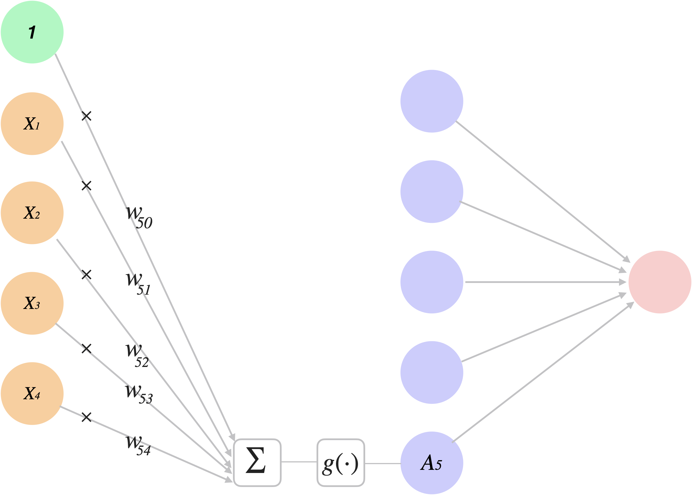
• In the terminology of neural networks, the four features \(X_1, \dots ,X_4\) make up the “units” in the input layer

• Each arrows feeds into each (\(k = 1, \dots K\)¹) of the so-called activations of the hidden layer : \[ A_k = h_k(X) = g(w_{k0} + \sum_{j=1}^p w_{kj}X_j) \] These \(A_k\)s are not directly observed, hence “hidden”.

• the “A” stands for activation
• each is a transformation of the inputs
• \(h_k\) is expanded to be a non-linear function of a linear combination of the inputs
• \(w_{k0}\) akin to intercepts (called bias)
• \(w_{kj}\) akin to \(\beta\) slopes (called weights)
• Note that each of these linear combinations is different
• Each \(h_k\) is different and are learned on the fly
• we also have a choice for these non-linear functions …

1. we get to pick \(K\); here we chose 5 but this is easily extended

The Model

The resulting model is then a linear combination in the \(K = 5\) activations:

\[ \begin{align} f(X) &= \beta_0 + \beta_1 A_1 + \beta_2 A_2 + \dots + \beta_K A_K\\ &= \beta_0 + \sum_{k=1}^K \beta_k h_k(X)\\ &= \beta_0 + \sum_{k=1}^K \beta_k g(w_{k0} + \sum_{j=1}^p w_{kj}X_j) \\ \end{align} \]

\(g(z)\) is typically a non-linear function (see activation functions) of \(z\), a linear combination of the inputs.

• so rather than performing linear regression on \(X_1, \dots, X_p\) we are performing them on activations \(A_1, \dots, A_K\)
• these activations are just non-linear functions of linear cobminations of the original data

Activation Functions

\(g(z)\) is called the activation function

• Sigmoid

• Tanh

• Relu

• LeakyReLU

• Softmax

A plot of the popular activation functions: the sigmoid function in green and rectified linear (or Relu) in black.

• RELU = rectified linear

• on the x-axis we have a standardized range for the linear transformations on X

• recall sigmoid was used in logistic regression to smoothly map the values from 0 to 1

• Relu = rectified linear unit The piecewise-linear ReLU function is popular for its efficiency and computability.

• analogous to neurons in the brain — values of the activations close to one are firing, while those close/equal to zero are silent

• why non-linear? if g was a linear function it would just be a really big linear model.

Sigmoid

In the early instances of neural networks, the sigmoid activation function was favoured:

\[ g(z) = \frac{e^z}{1+e^z} \]

Recall:

• the sigmoid function forms an S-shaped graph
• this was used in logistic regression to convert values on the real line into probabilities between zero and one

Relu

The preferred¹ choice in modern neural networks is the ReLU (rectified linear unit) activation function, which takes the form

\[ g(z) = \text{max}(0,z) = \begin{cases} 0 & \text{if }z<p\\ z & \text{otherwise} \end{cases} \]

Although it thresholds at zero, because we apply it to a linear function the constant term \(w_{k0}\) will shift this inflection point.

1. A ReLU activation can be computed and stored more efficiently than a sigmoid activation.

Common Activation Functions

Source of Image

• in practice RELU and softplus activations are commonly used
• best choice depend on the specific characteristics of the task, the nature of the data, and the architecture of the neural network.
• Experimentation and tuning are often required to identify the most suitable activation functions for a given application.

Summary of Single Layer NN

In summary, we derive five new features by computing five different linear combinations of \(X\), and then plug each through an activation function \(g(·)\) to transform it. The final model is linear in these derived variables and has the following parameters …

• Each arrow is associated with a weight, and the value of the weight determines the strength of the connection between the connected nodes.
• The weights are adjusted during training to learn the patterns in the data.
• so these arrows make up these linear combinations we’ve seen in the formula
• I rep bias as a separate node there

• linear combination of inputs where the \(w_{1i}\) can be thought of as regression coefficients and \(w_{i0}\) can be thought of like an intercept
• that linear combination is then passed through an activation function g
• note the subscripts are counter-intuitive (at least to me):
  • first subscript: the node it is feeding into in L1
  • second subscript: the input node that it is feeding from

• we do the same thing to get activation 2
• note that the same activation function \(g(\cdot)\) is typically used

• we do the same thing to get activation 4
• note that the same activation function \(g(\cdot)\) is typically used

** All these weights are going to be stored in a matrix called \(W\)**

• These 5 new activations can be thought of as new inputs for the next layer (at the end of the day they are non-linear transformations of the original X)
• all these \(\beta\)s are going to stored in a matrix called \(B\)

• finally, we get a linear combination of activations (i.e. hidden units) and pass it through some activation functions \(f(\cdot)\)
• Note: this function is different than the activation function used in the hidden layer (hence \(f\) instead of \(g\)). Choice depends on the task (eg. binary classification, regression, multiclass, etc)

Comment

• All hidden layers typically use the same activation function.

• The output layer will typically use a different activation function from the hidden layers.

• The \(w_{kj}\)s are the coefficients weights and \(w_{k0}\)s are the intercepts biases¹

• This is a “feed-forward neural network” - there are more complicated types of NN (e.g. backwards arrows, loops, no arrows)

• don’t have this strict sort of left to right graphical view
• we can feed some stuff forward
• some stuff might actually be back propagated through the network to sort of reinform estimations

1. not to be confused with the “bias-variance” usage elsewhere in course

Output Layer

Common choices for activations functions for the output layer:

1. Linear (aka “identity”)
   • multiplication by 1, i.e. no activation.
2. Sigmoid (aka “logistic”)
3. Softmax (for multi-class)
   • normalized exponential function which converts a vector of \(K\) real numbers into a probability distribution of \(K\) possible outcomes

Loss Function

In the regression¹ setting, for example, the model is fit by minimizing the familiar residual sum of squares:

\[ \mathcal{L} = \sum_{i=1}^n (y_i - f(x_i))^2 \]

This is commonly referred to as a loss function (or cost function, or objective function).²

• Note that \(f(X)\) which is at the end of the pipeline encompasses a LOT of parameters (which is quite characteristic of NN).
• The goal during training is to minimize this loss.
• we adjust the weights in the fitting process until to minimize the loss through backpropegation (common optimization algorithms include: Stochastic Gradient Descent (SGD) and variants like Adam)

1. for classification we might use cross-entropy

2. we will see how we can add L1/L2 Regularization later

Why Non-linear Activation Functions?

• The nonlinearity in the activation function \(g(·)\) is essential

• Without it the model \(f(X)\) would collapse into a simple linear model in \(X_1,...,X_p\).

• Moreover, having a nonlinear activation function allows us to capture complex nonlinearities and interaction effects.

• Let’s look at an example where the sum of two nonlinear transformations of linear functions can give us an interaction …

Example: Single Layer NN

Suppose we have two input variables \(X = (X_1, X_2)\), i.e. \(p=2\). In our hidden layer suppose we have two hidden units (i.e \(K=2\)) with activation function equal to \(g(z) = z^2\)

Suppose we have parameters: \[\begin{align*} \beta_0 &= 0, & \beta_1 &= \frac{1}{4} & \beta_2 &= - \frac{1}{4}\\ w_{10} &= 0, & w_{11} &=1 & w_{12} &= 1, \\ w_{20} &= 0, & w_{21} &=1 & w_{22} &= -1, \\ \end{align*}\]

we would not use a quadratic function for g(z), since we would always get a second-degree polynomial in the original coordinates

Example (activations)

The two activations in the hidden layer and then computed \[\begin{align*} A_k = h_k(X) &= g (w_{k0} + \sum_{j=1}^p w_{kj}X_j)\\ \end{align*}\]

\[ \begin{align*} A_1 &= h_1(X) \\ &= g (w_{10} + w_{11}X_1 + w_{12}X_2)\\ &= g (0 + 1\cdot X_1 + 1 \cdot X_2)\\ &= (X_1 + X_2)^2 \end{align*} \]

\[ \begin{align*} A_2 &= h_2(X)\\ &= g (w_{20} + w_{21}X_1 + w_{22}X_2)\\ &= g(0 + 1 \cdot X_1 + (-1) \cdot X_2)\\ &= (X_1 - X_2)^2 \end{align*} \]

Example (model)

Plugging \(h_1(X) = (X_1 + X_2)^2\) and \(h_2(X) =(X_1 - X_2)^2\) into the neural network model:

\[\begin{align*} f(X) &= \beta_0 + \sum_{k=1}^K \beta_k h_k(X) = \beta_0 + \beta_1 h_1(X) + \beta_2 h_2(X)\\ &= 0 + \frac{1}{4}(X_1 + X_2)^2 - \frac{1}{4} (X_1 - X_2)^2\\ &= \frac{1}{4}\left[ X_1^2 + 2\cdot X_1 X_2 + X_2^2 - (X_1^2 - 2 \cdot X_1 X_2 + X_2^2)\right] \\ &= X_1X_2 \end{align*}\]

• So the sum of two nonlinear transformations of linear functions can give us an interaction!
• so we no longer have to manufacture those interaction terms as we did before … just feed in the original data
• so these layers can discover interactions which is pretty powerful
• we would not use a quadratic function for \(g(z)\), since we would always get a second-degree polynomial in the original coordinates \(X_1,\dots , X_p\).
• Polynomial function whose general form is \(f(x)=Ax^2+Bx+C\)

Multilayer Neural Networks

• In theory¹ a single hidden layer with a large number of units has the ability to approximate most functions.

• However, the learning task of discovering a good solution is made much easier with multiple layers each of modest size.

• The weights \(w\) are parameters that require estimation. The quantity of these gets out of hand quickly.

• The adjective “deep” in deep learning refers to the use of multiple layers in the network.

• in the 80s NN typically had one hidden layer because of this proof that set the field back by 30 years
• Hence the new name of “deep learning” rather than neural networks
• not easy to interpret these layers
• you can think of these things as picking up certain aspects of the inputs
• lets look at an example

1. can be shown through approximation theorems

Digit Recognition Example

• Digit recognition problems were the catalyst that accelerated the development of neural network technology in the late 1980s at AT&T Bell Laboratories and elsewhere

• Turns out that these pattern recognition (that are relatively simple for humans) are not so simple for machines.

• It has taken more than 30 years to refine the neural-network architectures to match human performance.

Neural networks rebounded around 2010 with big successes in image classification. Around that time, massive databases of labeled images were being accumulated, with ever-increasing numbers of classes. (see 10.3 Convolutional Neural Networks CNN) - Success with RNNs (Recurrent neural network) for in speech and language translation, forecasting, and document modeling.

Digit Dataset

• The textbook goes through the process of setting up a large dense network on the famous and publicly available MNIST handwritten digit dataset (60K training, 10K testing)

• The idea is to build a model to classify the images into their correct digit class 0–9.

• Every image has \(p = 28 × 28 = 784\) pixels, each of which is an eight-bit grayscale value between 0 and 255 representing the brightness of a pixel (0 = black, 255 = white):

• different (yet the same) as the tabular data we’ve analyzed before
• These pixels are stored in the input vector X (in, say, column order).
• The output is the class label, represented by a vector Y = (Y0, Y1,…,Y9) of 10 dummy variables, with a one in the position corresponding to the label, and zeros elsewhere.
• we haven’t done any multi response stuff in this course yet (so may be a stretch)

Example images

• hidden layer neurons try to add up little patterns in these drawings to “fire” the pathway that points to the correct classification
• note this model requires us to standardize the images (all 28x28 grayscale)
• it’s mostly just a black box though
• the NN is just a function where each neuron is a sub function function and fitting it comes down to estimating the weights and biass such that your outputs make sense
• 4 times as many paramters as observations FLAG: overfitting?

Two-Layer Feed-forward NN

ISLR Fig 10.4. Neural network diagram suitable for the MNIST handwritten-digit problem. The input layer has \(p\) = 784 units, the two hidden layers having \(K_1 = 256\) and \(K_2 = 128\) units respectively, and 10 output layer units. Along with intercepts (AKA biases) this network has 235,146 parameters (aka weights).

Parameters:

• two hidden layers (L1 and L2) instead of one (this is an example of a “deep” net vs. the “shallow” network from before)
• it has 784 (28x28 = 784) input nodes (number of pixels in image)
• it has 10 output variables in the output layer (0,1,..9)
• 235, 146 parameters total (60K in the training set- 10K in test)

The number layers is a choice we make before the model is trained

• in NN one of the first things you do is decide how many hidden layers you want and how many activation nodes go into each hidden layer.
• although there are rules of thumb for making decisions about the hidden layers, you essentially make a guess and see how well the neural network performs, adding more layers and nodes if needed.

Arrows

• \(w_{\ell j}^{1}\) and \(w_{\ell j}^{2}\) are weights and \(w_{k0}\) is the bias term

• each arrow represents all the weights going from every input to every hidden unit

• likewise we have a second hidden layer which takes the values from the first hidden layers as inputs

Ouput layer

• will give a probability of the digit being a 0, 1, … 9 and those lead to a prediction (used the softmax activation function)

First Hidden Layer

The first hidden layer takes a linear combination 784 inputs stored in \(X\) as inputs for the activation function. For \(k = 1, \dots, K_1 = 256\) we have: \[\begin{align*} &A_k^{(1)} = h^{(1)}_k(X) = g (w^{(1)}_{k0} + \sum_{j=1}^{p = 784} w^{(1)}_{kj}X_j) \end{align*}\]

• \(W_1\) is the 785 \(\times\) 256 matrix of weights that feed from the input layer to hidden layer one (L1),
• i.e. \(W_1 = \{w_{kj}^{(1)}\}\), \(j =\) 0, 1, \(\dots p\), and \(k=1, \dots, K_1\)

• 256 nodes or units in our first layer, p is 784
• 785 rather than 784 since we must account for the intercept or bias term \(w_{k0}\)

Second Hidden Layer

The second hidden layer takes a linear combination of the activations \(A_k^{(1)}\) from the first hidden layer as inputs for the activation function. For \(\ell = 1, \dots, K_2= 128\) we have: \[\begin{align*} &A^{(2)}_\ell= h^{(2)}_\ell(A_k^{(1)})= g (w^{(2)}_{\ell 0} + \sum_{k=1}^{K_1=256} w^{(2)}_{ \ell k}A_k^{(1)}) \end{align*}\]

• \(W_2\) is the \(25\textbf{7}\times 128\) matrix of weights that feed from the first hidden layer (L1) to the second hidden layer (L2),
• i.e. \(W_2 = \{w_{\ell k}^{(2)}\}\), with \(k=\textbf{0}, \dots, K_1\) and \(\ell = 1,\dots K_2\)

• Thus, through a chain of transformations, the network is able to build up fairly complex transformations of X that ultimately feed into the output layer as features.
• again we have 257 instead of 256 becuase we have an extra intercp term (aka bias)

Output Layer

The output layer takes a linear combination of these activations \(A_\ell^{(2)}\) from the second hidden layer as inputs and for output activation function. For \(m = 0, \dots, 9\): \[\begin{align*} f_m(A_\ell^{(2)}) &= f_m \left( \beta_{m0} + \sum_{\ell=1}^{K_2 = 128} \beta_{m\ell} A_\ell^{(2)} \right) \end{align*}\]

• \(B\) is the \(12\textbf{9} \times 10\) matrix of weights that feed from the second hidden layer (L2) to output layer,

• i.e. \(B = \{ \beta_{m \ell} \}\) with \(\ell = \textbf{0},\dots K_2\), and \(m=0, \dots, 9\)

Softmax

• As stated previously, the output layer typically use a different activation function from the hidden layers

• The output activation function used here is the softmax function which returns probabilities i.e. \(\sum_{m=0}^9 f_m(X) = 1\): \[\begin{equation} f_m(X) = \text{P}(Y=m \mid X) = \frac{e^{Z_m}}{\sum_{\ell=0}^9 e^{Z_{\ell}}} \end{equation}\] where \(Z_m = \beta_{m0} + \sum_{\ell=1}^{K_2} \beta_{m\ell}A_\ell^{(2)}\). We assign the image to the class with the highest probability.

• \(Z_m\) is ten linear combinations of activations at the second layer.
• same function that is used in multi-class logistic regression

Cross-entropy

We fit the model by minimizing the negative multinomial log-likelihood, or cross-entropy¹:

\[ \mathcal{C} = \begin{equation} - \sum_{i=1}^n \sum_{m=0}^9 y_{im} \log (f_m(x_i)) \end{equation} \]

where \(y_{im}\) is 1 if the true class for observation \(i\) is \(m\), else 0. These classes are said to be one-hot encoded²

• You add up the log of the predicted probabilities to the assigned class (the probability of belonging to a class that it was not assigned to get multiplied by 0)
• we like to use \(m-1\) dummy variables (one hot has a variable for each level)

1. as with regression, this is alternatively referred to as a loss function or cost function

2. this is closely related to dummy variables

Dummy variables One-hot encoding

• Like the regression model, NN will require that our categorical data be converted to numeric form.

• When no ordinal relationship exists we use one-hot encoding which encodes \(N\) categories using binary (aka dummy) variables

Original	red.dummy	green.dummy	blue.dummy
red	1	0	0
green	0	1	0
blue	0	0	1

while we could covert each class to an integer (in the case of this digit example, we could just use the numeric digits the images represent) however this assumes a natural ordering

Number of Parameters Weights

• This model has 235,146 parameters (referred to as weights):
  • \(W_1\) has \(785×256 = 200,960\) weights¹
  • \(W_2\) has \(257 × 128 = 32,896\) weights\(^1\)
  • \(B\) has \(129×10 = 1290\) weights\(^1\).

Note that we have close to 4 times as many parameters as we do training observations (60k).

What should we be concerned about?

when \(p>n\) (like in LASSO/Ridge) what are we susceptible to? - overfitting!

1. the additional row for each weight matrix accounts for the intercept bias terms \(w_{\cdot 0}\)

Overfitting

• One of the most important aspects when training neural networks is avoiding overfitting.

• To avoid overfitting, some regularization is needed.

• As in our regression unit, regularization will be achieved by adding a penalty term regularization term to our loss function in order to penalize complexity.

• This will effectively shrink (or remove) certain weights thereby making some hidden neurons negligible and reducing the overall complexity of the NN.

• these models are very flexible and will tend to overfit
• In short: Less complex neural networks are less susceptible to overfitting. To prevent overfitting or a high variance we must use something that is called regularization.
• smoothing or droping out weights

Regularization

Two popular regularization techniques are:

1. L1 regularization (aka LASSO regularization)
2. L2 regularization (aka Ridge regularization)

As you may be able to guess, L1 regularization forces the weights to become (exactly) zero and L2 regularization forces the weights towards (but never exactly) zero.

L1/L2 Regularization

• L2/Ridge regularization uses the L2 norm \(|| W ||_2^2\) in it’s regularization term¹ and adds it to the loss function: \[ \mathcal{L} + \frac{\alpha}{2}|| W ||_2^2 \]

• L1/LASSO regularization uses the L1 norm \(|| W ||_1\) in it’s regularization term\(^1\) and adds it to the loss function: \[ \mathcal{L} + \alpha|| W ||_1 \]

1. where \(\alpha\) is the regularization rate.

Dropout

Another powerful option is dropout regularization.

Figure source: DeepLearning.AI YouTube video

Simply put, we created a smaller network by removing nodes according to some probability (in this case \(p =0.5\)).

• DeepLearning.AI founder Andrew Ng, Chairman and Co-Founder of Coursera and an Adjunct Professor at Stanford University’s Computer Science Department.
• a neural network diagram where with three hidden layers. On the left we have a feedforward neural network with no dropout. On theright we have some of the nodes in these hidden layers have an x through them, indicated that they are dropped from the network

Results

Method	Test Error
Neural Network + Ridge Regularization	2.3%
Neural Network + Dropout Regularization	1.8%
Multinomial Logistic Regression	7.2%
Linear Discriminant Analysis	12.7%

This is a historic example that marks one of the early “wins” for neural networks in the 1990s.

• substaintial improvements
• very overworked problem – best reported rates 0.5%
• human error rate 0.2%

Training NN

• Once the structure is determined, we’re left with a non-linear optimization problem.

• Typically, NNs are trained using the stochastic gradient descent and weights are updated using the backpropagation.

• We will give a brief overview using the loss function for regression but these ideas can be extended to classification and to when Regularization penalties are applied.

• constraints or the objective function are nonlinear

• we cant use the techniques we used for OLS for example

• an algorithm searches the space of possible sets of weights

Single Hidden Layer Revisited

• Lets return to the Single Hidden Layer example used in our first network diagram.

• In this model the parameters are \(\beta = (\beta_0, \beta_1. \beta_K)\), as well as each of the \(w_k = (w_{k0}, w_{k1,}...,w_{kp})\), for \(k = 1, . . . , K\).

• Given observations \((x_i, y_i)\), for \(i = 1, \dots, n\) we could fit the model by minmizing the loss function with respect to the parameters, \(\beta\), and \(W\).

Why we need Gradient Decent

While this might look like the minimization problem we had in linear regression, the following is not straightforward to minimize. \[ \mathcal{L}(\beta, W) = \sum_{i=1}^n (y_i - f(x_i))^2 \]

Furthermore, this problem is nonconvex in the parameters, and hence there are multiple solutions.

Gradient Descent

• At the basic level, we adjust the weights so that error is reduced for the next iteration.

• More technically, the optimization algorithm is navigating down the gradient (or slope) of error and seeks to change each weight proportionally to its effect on the RSS: \[\begin{equation} \Delta w_{\cdots} = - \alpha \frac{ d RSS}{d w_{ \cdots}} \end{equation}\] where \(\alpha\) is a learning rate.

• visualize that you are randomly placed on a mountainous terain, (Start with an itial guess for the parameters.)
• We need to make it to the bottom of the mountain so we continue to take steps downhill
• the correct directions are determined by gradient decent, find the partial derivatives and plug in your current guess– this gives the direction which increases most rapidly (and we move in the opposite direction)
• when the gradient vector is zero, we have arrived at a minimum
• The the derivative w.r.t. the parameters to figure
• global solution is not unique

backpropagation

1. chain rule to calculate derivatives
2. plugging derivatives into gradient decent to optimize parameters

Gradient Descent Algorithm

1. Take the derivative of the loss function for each parameter (i.e. find the gradient for the loss function)
2. Pick random values for parameters
3. Plug in the parameters values into the derivatives (i.e. gradient)
4. Calculate \(\text{Step Size} = - \alpha \frac{ d RSS}{d w_{ \cdots}}\)¹
5. Update: New Parameters = New Parameters + Step Size

• step size = derivative of the slop of the error at that current value of \(w\) times the learning rate

1. Since this takes a long time with large \(n\) we instead used stochastic gradient decent that randomly selects a subset (i.e. mini-batch) of the data at every step

Non-convexity

ISLR Fig 10.7: Illustration of gradient descent for one-dimensional \(\theta\). The objective function \(R(\theta)\) is not convex, and has two minima, one at \(\theta = -0.46\) (local), the other at \(\theta = 1.02\) (global). Starting at some value \(\theta_0\) (typically randomly chosen), each step in θ moves downhill — against the gradient — until it cannot go down any further. Here gradient descent reached the global minimum in 7 steps.

Learning Rate

• The learning rate is akin to that which we saw in Boosting.

• Essentially it is included so that the alorithm “learns slow” and avoids overfitting.

• Typically this value is very small (say ~0.1)

• The algorithm will be highly dependent on this value and often it’s set to “schedule” that starts off large and gets smaller and smaller.

Backpropagation

• Geoffrey Hinton, David Rumelhart and Ronald J. Williams pioneered the back-propagation algorithm in a pair of landmark papers published in 1986.

• As a very briefoverview, we work out way through the NN backwards (hence the name), and computes the gradient

• stochastic gradient descent, is then used to perform learning using this gradient.

• backpropagation neural networks become so efficient
• two of those are from Jason Brownlee who i find writes really good articles in machine learning

Together, the back-propagation algorithm and Stochastic Gradient Descent algorithm can be used to train a NN. Helpful links - ISLR2 Ch 10.7, tds (Jason Brownlee), StatQuest, machinelearningmaster (Jason Brownlee), LeCun paper

Visualization of Backpropigation

Source of Image

Epoch in NN

• An epoch is completed each time the algorithm sees the all the samples in the dataset in a cycle (i.e. a forward pass and a backward pass).

• An epoch is made up of one or more batches (or mini-batches), where we use a part of the dataset to train the neural network.

• An iteration is completed each time a batch of data passed through the algorithm (i.e. a forward pass and backward pass).

• The number of epochs is a hyperparameter that the user must specify before training the model.
• An iteration, on the other hand, refers to one update of the model’s weights. In the context of training, an iteration corresponds to processing one mini-batch of training examples and updating the model’s parameters based on the calculated gradients.

Huh?

• the confusion arrises since we don’t use all that training data at each pass.
• iteraction for mini-batches
• epochs for complete data (aka “batch” where a batch is the complete dataset. – which is confusing since it is also used as a synonym for mini-batch)

Batches in NN

For each epoch, the required number of iterations times the batch size gives the number of data points.

• An epoch is sometimes mixed with an iteration.
• usually there are multiple interations per epoch
• right example 10 iterations per epoch

Network Tuning

Fitting NN requires a number of choices that all have an effect on the performance:

• The number of hidden layers, and the number of units (or nodes) per layer.

• Regularization technique/ tuning parameters

• Details of stochastic gradient descent

• choice of activation functions

These choices can make a big difference. The tinkering process can be tedious, and can result in overfitting if done carelessly.

TensorFlow Playground

• You can play around with this in the TensorFlow Playground

• You can set the regularization (L1/L2 for LASSO/Ridge, respectfully)

NN in R

• One popular way of fitting Neural Networks in R is to use the keras package¹

• It can be a bit finicky to install our your computer but you follow this instructions from the textbooks website here

• This package interfaces to the tensorflow package which in turn links to efficient python code.

• For this course, we’ll just stick to the neuralnet and NeuralNetTools packages for our simple demonstrations.

• python is a popular programming language (esp. in ML)

1. Deep Learning with R is a helpful text (but probably better to move to python)

Example: Body NN

• We fit a neural network with one hidden layer, four hidden layer nodes (or neurons/units) to predict recorded Gender.

library(gclus)
data(body)
sbod <- cbind(scale(body[,1:24]), factor(body[,25]))
colnames(sbod)[25] <- "Gender"
# load the pacakge for Neural Networks
library(nnet)
# size = nodes in hidden layer
# fits a single layer NN
nnbod2 <- nnet(factor(Gender)~., data=sbod, size=4)

We call to another package to produce a plot for it …

• This dataset contains 21 body dimension measurements as well as age, weight, height, and gender on 507 individuals. The 247 men and 260 women were primarily individuals in their twenties and thirties,
• Fit single-hidden-layer neural network

Plotting the NN

library(NeuralNetTools);  plotnet(nnbod2)

read next slide

Properties of the Network Digaram

• For NeuralNetTools package, positive weights show up as black, negative as grey.

• Also the biases are shown as a separate node (B1 and B2) on the graph; for simpler NN, the weights would be shown on the lines connecting the nodes.

• In this case, the magnitude of the weight shows up as the thickness of the line.

• There are 25 (24 predictors + 1 bias term) x 4 (hidden layer units) + 5 (hidden layer units + 1 bias term) x 1 (output layer unit) = 105 weights

Example: Body NN

• How does it perform??

table(body[,25], predict(nnbod2, type="class"))

   
      1   2
  0 260   0
  1   1 246

• 0 misclassifications!

But of course, this is on the training set, so let’s do a training/testing set to approximate the long-run error.

• Are you properly predicting your error (through CV or training/testing), or are you reporting error from the set you trained on?
• In simpler form: are you overfitting???

Validation Approach with Body NN

• Set up a quick training and testing set. Sample approx half the data for a 50-50 training/testing scenario, refit 4 hidden variable NN to the training set, and predict on the test set…

set.seed(53747958)
bindex <- sample(1:nrow(sbod), nrow(sbod)*.50)
btrain <- sbod[bindex,]
btest <- sbod[-bindex,]
nnbodtr <- nnet(factor(Gender)~., data=btrain, size=4)

table(btest[,25], predict(nnbodtr, newdata=btest[,-25], type="class"))

   
      1   2
  1 122   2
  2   4 126

6 misclassifications and misclassification rate of 0.023622

Example: Body NN

• How does that compare to some of our other methods?

• RF on same train/test? Misclassify 21. Rate closer to 8%. NN wins that battle.

• LDA on same train/test? Misclassify 6. Rate closer to 2%. And it’s a much simpler model for interpretation.

• So, be careful. Trendy, flexible models are not a cure-all. They need to be carefully tuned and tested.

• with some tweaking we can do just as good, but why would we? we have a simplier model that does good already
• lda is easier to interpre (eg means of gender)

Taking it further

Different types of data call for different variations. For example

• ISLR2 Ch 10.3 - CNN (Convolutional Nueral Networks) are a special family of NN for classifying images and video (see ISLR2 Ch 10.3)
• ISLR2 Ch 10.4 - the bag-of-words model can be used for predicting attributes of documents
• ISLR2 Ch 10.5 - RNN (Recurrent Neural Networks) are used when data are sequential in nature (e.g. time series, documents)

• we don’t have time to go over the architecture but see ISLR2 ch 10.3

CNN - the convolution fitler slides around the image score for matches using dot products Document Classification

bag-of words - Dictionary of \(M\) words we score each document for the presence or absence of each of the words

CNN

• since we can parallize the process this will be able to do this quickly.
• CNN major success story for classifying images (can usu color images with a R/G/B chanels rather than just a single grayscale - so 3D)
• CNN Builds up an image in a hierarchical fashion, finds small local edges and shapes eventually assembling the target image
• these filters are learned
• You can used pre-trained CNN classifies (eg. resnet50 classifier was trained using the imagenet date set, which consists of millions of images that bloeng to an ever-growing number of categories)
• using these pre-trained hidden layes can save you days of training

Summary

Pros

• Powerful predictive tools
• Parellization
• Easily extended to multiple response models
• Can use pre-trained NN

Cons

• Black box (lack of interpretibility)
• Lots of tuning to consider
• High danger of overfitting
• Requires very large training set