Data 311: Machine Learning

Lecture 15: Boosting

Dr. Irene Vrbik

University of British Columbia Okanagan

Recap

• Last time we saw how bootstrap aggregation (or bagging) can be used to improve decision trees by reducing its variance.

• For Random Forest (RF) we use a similar method to bagging, however, we only consider m predictors at each split¹.

• That added randomness in RF further reduce the variance of the ML method, thus improving the performance even more.

1. for classification we usually use \(m = \sqrt{p}\) and for regression we use \(m = p/3\)

Introduction

• We now discuss boosting, yet another approach for improving the predictions resulting from a decision tree

• Again, we focus on decision trees, however, this is a general approach that can be used on many ML methods for regression or classification.

• Like bagging and random forests, boosting involves aggregating a large number of decision trees; that is to say, it is another ensemble method.

From bagging to boosting

Some differences moving from bagging to boosting:

1. no more bootstrap sampling
2. trees are grown sequentially (as opposed to in parallel)
3. trees are added together rather than averaged.
4. rather than fitting “bushy” trees we prefer “stumps”

Boosting is a fairly simple variation on bagging that strives to improve the weak learners by focusing on areas where the system is not performing well.

Bagging

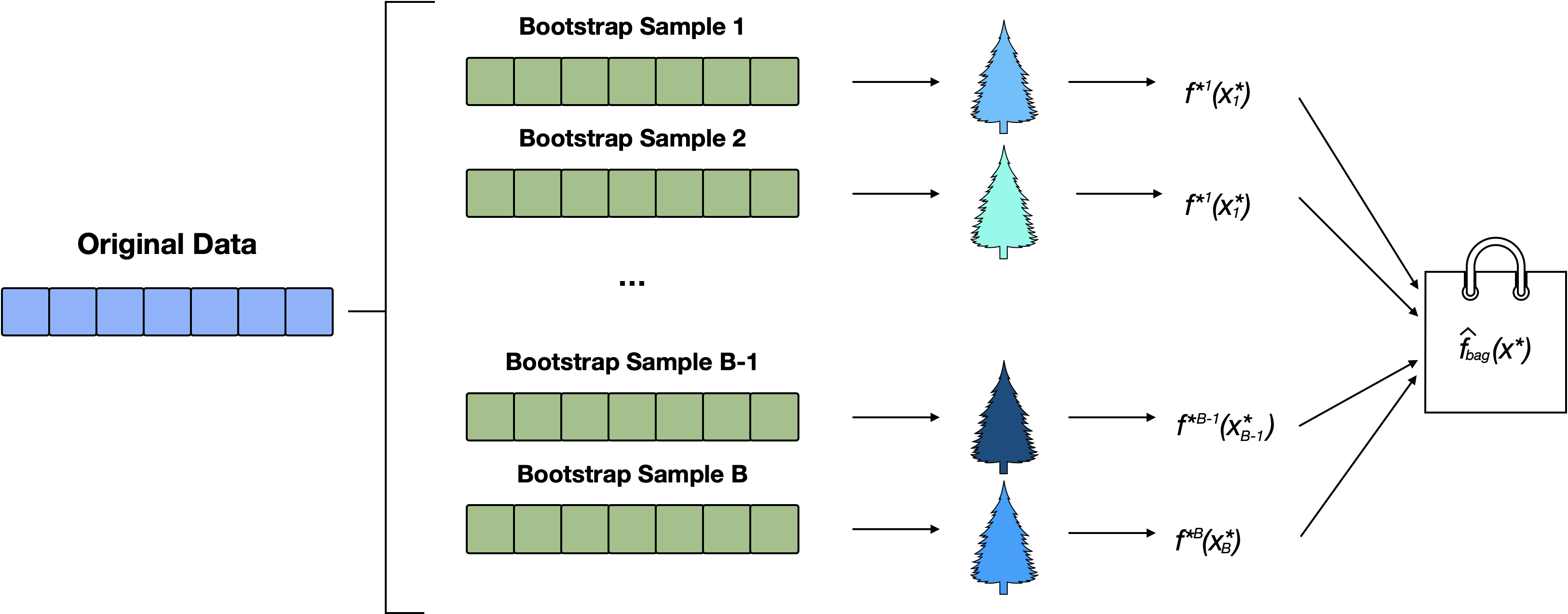
Bagging is an ensemble algorithm that fits multiple multiple trees on different bootstrap samples, then combines the predictions from all models in a single bagged prediction.

• we get some variation due to the nature of bootstrapping, but the trees may look somewhat similar
• N.B trees are grown independently on random samples of the observations. IOW, a random reshuffling of the bootstrap samples won’t make a difference since each tree is fitted in parallel

Random Forests

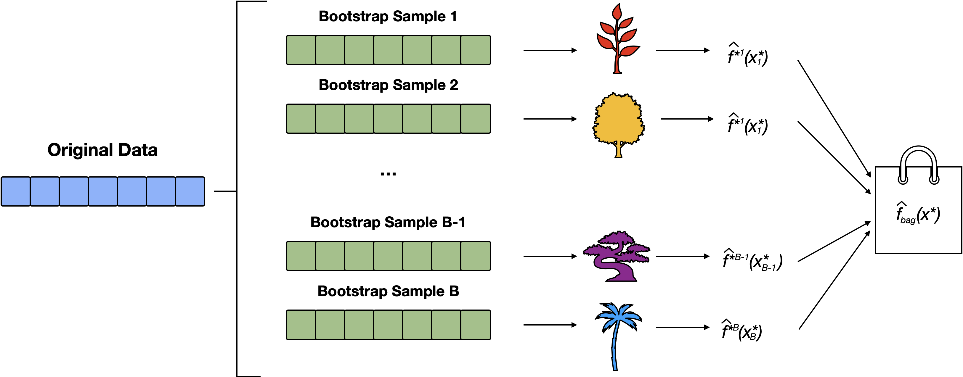
Random forest is an extension of bagging that randomly selects subsets of predictors at each split (thereby diversifying the forest)

• Random forest is an extension of bagging that randomly selects subsets of predictors at each split (thereby diversifying the forest)
• average the predictions from these trees to reduce variance
• again these trees are fit in parallel

From Bushy Tree to Stumps

• You may recall that when we make a RF, we fit full sized (aka bushy) trees.

• Note that these trees (by design) may look quite different from one another (i.e. they will have difference decision rules, different sizes, etc…)

• In boosting, we make a forest of “short” trees (eg. \(d\)¹= 1, 4, 8, 32); maybe having one node and two leaves (aka stumps)

• These stumps are referred to as a “weak learners”²

• Weak Learner will be preferable to the boosting method which “learns slow” by additing these weak learnings together.

1. where \(d\) is the number of decision rules (see Boosting Tuning Parameters)

2. simple models that do only slightly better than random chance

Boosting stumps

Note Difference:

bagging involves:

• bootstrap, fitting a separate decision tree in parallet, combining all answers to a single predictive modle.

Boosting works in a similar way, except:

• does not involve bootstrap sampling;

• instead eachtree is fit on a modified version of the original data set.

Bye-bye boostrap

• Boosting does not involve bootstrap sampling; instead each tree is fit to the residuals obtained from the last tree.

• That is, we fit a tree using the current residuals, rather than the outcome \(Y\), as the response.

• This approach will “attack” large residuals, i.e. will focus on areas where the system is not performing well.

Boosting vs. Bagging/RF

Apart from the boostrap samples, there are other important differences between boosting and random forests:

• Trees will be grown sequentially such that each tree will be influenced by the tree grown directly before it.

• Like RF, boosting involves combing a larger number of decision trees \(\hat f_1, \dots, \hat f_B\), however…

• rather than taking the average (or majority vote) of the corresponding predicted values, the combined prediction is typically a weighted average (or a voting mechanism).

• the weight is going to reflect how well that tree performed.
• learners that perform better are given more weight in the final prediction.

how do we bring these trees together?

Benefits

• Improved Accuracy: By focusing on previously misclassified data points, boosting reduces bias and helps the model fit the training data more accurately.

• Reduced Overfitting: Boosting also reduces the risk of overfitting, as it combines the predictions of multiple weak learners, which helps generalize the model.

• Robustness: It can handle noisy data and outliers because it adapts to misclassified points.

• Unlike fitting a single large deci- sion tree to the data, which amounts to fitting the data hard and potentially overfitting, the boosting approach instead learns slowly.

How to ensemble

• By fitting small¹ trees to the residuals, we slowly improve \(\hat f\) in areas where it does not perform well.

• To slow this down even further, we multiple this fit by a small positive value set by our shrinkage parameter \(\lambda\).

• We then add this shrunken decision tree into the fitted function to produce a small incremental nudge in the right direction

• In general, statistical learning approaches that “learn slowly” tend to perform well

• try to pick up a small peice of the signal with each subsequent tree

1. with just a few terminal nodes, determined by the parameter \(d\) in the algorithm.

Algorithm

1. Set \(\hat f(x)=0\) and \(r_i =y_i\) for all \(i\) in the data set \((X, r)\).
2. For \(b= 1,\dots, B\), repeat:

   1. Fit a tree \(\hat f_b\) with \(d\) splits (\(d+1\) terminal nodes) to \((X,r)\)

   2. Add a shrunken version off this decision tree to your fit: \[\begin{equation} \hat f(x) = \hat f(x) + \lambda \hat f_b(x) \end{equation}\]

   3. Update residuals \(r_i = r_i - \lambda \hat f_b(x)\)

3. Output the boosted model \(\hat f(x) = \sum_{b=1}^B \lambda \hat f_b(x)\)

1. Start off with a short tree (maybe one decision node) on the original data

2.1. replace y with r and fit as normal (but don’t go all the way to bushy tree-stop when number of terminal notes is d+1) 2.2. so we shift our prediction slowly towards some direction

• we slowly improve \(\hat f\) in areas where it does not perform well.
• λ slows the process down, allowing more and different shaped trees to attack the residuals.
• notice how the tree relies on the outcomes of the previous tree
• no bootstrap sampling needed

Details on boosting for classification appears in Ch 10 of ESL (more complicated). Both problem can be handled with the gbm (gradient boosted model) package

Gene expression Data

Results from performing boosting and random forests on the 15-class gene expression data set in order to predict cancer versus normal. The test error is displayed as a function of the number of trees. For the two boosted models, \(\lambda\) = 0.01. Depth-1 trees slightly outperform depth-2 trees, and both outperform the random forest, although the standard errors are around 0.02, making none of these differences significant. The test error rate for a single tree is 24 %.

• A very simple model applied in a slow and sequential way with predict very well.
• typically one will try a few values of d (mabye 1,2,4, 8 )
• you can see a sort of leveling off which is typical in these classification problems,
• however it is possible to overfit if we set B too large
• some in some problems you could see this test error go up after a certain point (this is unlike bagging and rf)
• typically one will try a few values of d (mabye 1,2,4, 8 )
• unlike RF we can overfit, although it would take a really long time for that to happen.

Boosting Tuning Parameters

Boosting requires several tuning parameters:

• \(B\) = the number of fits (trees for today’s example)

  • Unlike bagging/RF, boosting can overfit if \(B\) is too large¹

• \(\lambda\) = learning rate for algorithm, a small positive number

  • e.g. 0.01 or 0.001 are common

• \(d\) = complexity or interaction depth (often \(d=1\) works well)

  • for trees, this is the number of rules (i.e. internal/decision nodes) so \(d+1\) is the number of terminal nodes.

• if the model is very simply \(\lambda\) will have to be pretty small (if the model is dumb it will take longer to learn) and need more trees
• if the model is more complex \(\lambda\) can be bigger and therefore learn quicker
• tune this using cross-validation
• Very small λ can require using a very large value of B in order to achieve good performance.

1. We use cross-validation to select \(B\).

Example: Regression Simulation

Recall the regression simulation from our CART lecture:

head(dat)

Step 1:

Set \(\hat f(x)=0\) and \(r_i =y_i\) for all \(i\) in the data set \((X, y)\).

colnames(dat) <- c("X", "r"); head(dat)

Step 2a:

For \(b= 1,\dots, B\), fit a tree \(\hat f_b\) with \(d\) splits (\(d+1\) terminal nodes) to \((X,r)\)

fhat =  rep(0, nrow(dat))
lambda <- 0.005; B = 700; d = 1
for(i in 1:B){
  regt <- tree(r~X, data=dat, control=
                 tree.control(nobs = nrow(dat), mincut = 2, 
                    minsize = 4, mindev = 0.001))
  stump <- prune.tree(regt, best=d+1)
}

see ?tree.control():

• mincut = min obs to include in children nodes (default 5)
• minsize = smallest allowed node size (default 10)
• mindev = within-node deviance must be at least this times that of the root node for the node to be split (default = 0.01)

\(\hat f_1(x)\)

Step 2b:

… add a shrunken version off this decision tree to your fit:

fhat =  rep(0, nrow(dat))
lambda <- 0.005; B = 700; d = 1
for(i in 1:B){
  regt <- tree(r~X, data=dat, control=tree.control(nrow(dat), 2, 4, 0.001))
  stump <- prune.tree(regt, best=d+1)
  fhatb = predict(stump)
  fhat <- fhat + lambda*fhatb
  # ... more to do
}

\[\begin{equation} \hat f(x) = \hat f(x) + \lambda \ \hat f_b(x) \end{equation}\]

Shrunken Tree

\(\hat f(x) = 0 + \lambda \hat f_1(x)\)

Step 2c:

… update residuals \(r_i = r_i - \lambda \ \hat f_b(x)\)

fhat =  rep(0, nrow(dat))
lambda <- 0.005; B = 700; d = 1
for(i in 1:B){
  regt <- tree(r~X, data=dat, control=tree.control(nrow(dat), 2, 4, 0.001))
  stump <- prune.tree(regt, best=d+1)
  fhatb = predict(stump)
  fhat <- fhat + lambda*fhatb
  dat$r <- dat$r - lambda*fhatb
}

Updated residuals

\(r_i = r_i - \lambda \hat f_1(x)\)

Set \(b = b + 1\), rinse and repeat.

this might look the same but it’s actually the residuals

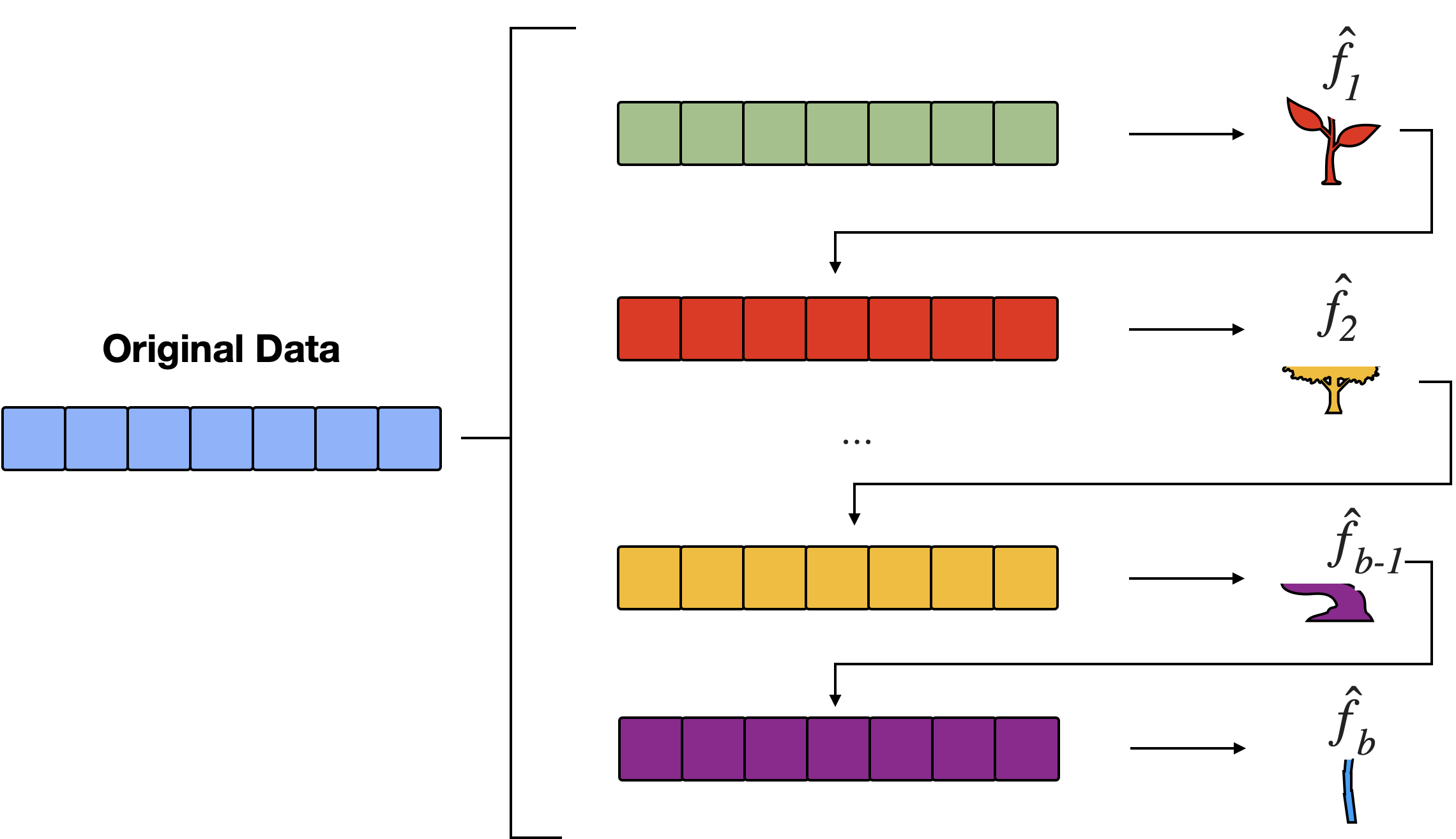
Algorithm Visualization

Top: current stump:

• best = 2 terminal nodes in prune.tree N.B. If there is no tree in the sequence of the requested size, the next largest is returned (so there are some trees with 3 terminal nodes, i.e. d = 2)

Bottom fitted function: \(\hat f(x) = \hat f(x) + \lambda \hat f_b(x)\)

Main ideas: - Learns slowly (this is every 10th iteration) - starts by attacking that high residual that big jump that corresponded to our root node in our original regression tree (thats going to be the case for a while) - at each iteration we’re trying to pick up a little piece of the signal

Algorithm Comments

• Given the current model, we fit a decision tree to the residuals (each tree relies on the previous tree)
• We then add a shrunken version of this decision tree to the fitted function \(\hat f\) (to nudge it a bit in the right direction)
• Each tree can be rather small (determined by \(d\))¹

By fitting small trees to the residuals, we slowly improve \(\hat f\) in areas where it does not perform well.

1. \(d\) = 2 in our case, however if there is no tree in the sequence of the requested size, the next largest is returned (so you may see some trees with 3 terminal nodes)

Step 3

Output the boosted model \(\hat f(x) = \sum_{b=1}^B \lambda \hat f_b(x)\)

• this crashes sometimes (code in lab)
• actually goes much slower as this is showing every 10th tree
• this additions can be negataive
• 700 trees plots every 10

Boosting for classification

• Boosting for classification is similar in spirit to boosting for regression, but it is a bit more complex

• We will not go into detail here, nor does the ISLR book

• Interested students can learn about the details in Elements of Statistical Learning, Chapter 10

• To perform boosting with trees (both in the classification and regression setting), we can use the gbm() (gradient boosted models) function from the gbm package.

Boosting function

library(gbm)
gbm(formula, distribution = "bernoulli", n.trees = 100,
  interaction.depth = 1, shrinkage = 0.1)

• distribution = “bernoulli” (for binary 0-1 responses), “gaussian” (for regression), “multinomial” for multi-class

Tuning parameters:

• interaction.depth = \(d\),
• shrinkage = \(\lambda\)
• n.trees = \(B\).

You can overfit here, so play around with these

Comments about gbm

• While this is the function that is used for boosting in the textbook, when you do boosting for a multi-class classification problem you will get the warning that:

Setting distribution = "multinomial" is ill-advised as it is currently broken. It exists only for backwards compatibility. Use at your own risk.

• Other package options exist (eg. tree booster in Extreme Gradient Boosting xgboost instead)

• XGBoost is known for its computational efficiency
• highly optimized, making it faster and more scalable compared to GBM
• However it uses Regularization: XGBoost includes L1 (Lasso) and L2 (Ridge) which makes it less interpretible

Example: Wine

Let’s perform boosting on the wine data set from the gclus package. As this is a multi-class classification problem, be advised that running this will produce a warning.

library(gbm)
library(gclus); data(wine)
weak.lrn <- gbm(factor(Class)~., distribution="multinomial",
              data=wine, n.trees=5000,
              interaction.depth=1)

Example: Wine

To get a sense of the test error and compare with bagging and RF, we can again use a cross-validation approach (here LOOCV)

library(gbm)
library(gclus); data(wine)
cvboost <- NA
for(i in 1:nrow(wine)){
  # preform boosting on the cross-validation training set
  weak.lrn <- gbm(factor(Class)~., distribution="multinomial",
                data=wine[-i,], n.trees=5000,
                interaction.depth=1)
  # Prob x_i belongs to the g = 1, 2, 3 group
  pig = predict(weak.lrn, n.trees=5000,
                newdata=wine[i,], type="response")
  # predict the class for the ith validation observation
  cvboost[i] <- which.max(pig) 
 }

• takes some time to run
• I had to cache the results from this chunk

CV error rate

   cvboost
     1  2  3
  1 58  1  0
  2  1 70  0
  3  0  0 48

This cross validated error rate is 1.12%. In this case boosting is equivalent to RF in terms of prediction. Recall:

RF (1.12%) > Bagging (3.37%) > Simple Tree (8.43%).

very good results for this data

Example: body

Recall the body data from the gclus pacakge:

• It contains 21 body dimension measurements as well as age, weight, height, and gender on 507 individuals;

• so \(p = 24\) (treating gender as our binary response)

1. Fit boosting using the validation approach (train/test) to obtain est of err
2. Fit RF and obtain the OOB error est
3. Compare est of eff from train/test (3.29) with cross-validated (1.38)

body: Boosting

set.seed(45613)
library(gbm); data(body) # code doesn't work is Gender is factor
train <- sample(1:nrow(body), round(0.7*nrow(body)))
bodyboost <- gbm(Gender~., distribution="bernoulli", data=body[train,],
                n.trees=5000, interaction.depth=1)
pprobs <- predict(bodyboost, newdata=body[-train, ], type="response",
                  n.trees=5000) 
(boosttab <-  table(body$Gender[-train], pprobs>0.5 ))

   
    FALSE TRUE
  0    74    0
  1     5   73

Test misclassification rate is 3.29%

Let’s use gbm to apply boosting to the body data with 5000 trees, with trees up to depth 1

• validation approach is subject to a lot of variabiliy so lets do cv
• improvement will level out; see last example ISLR lab

body: Random Forests

set.seed(4521)
library(randomForest)
(bodyRF <- randomForest(factor(Gender)~., data=body, importance=TRUE))

Call:
 randomForest(formula = factor(Gender) ~ ., data = body, importance = TRUE) 
               Type of random forest: classification
                     Number of trees: 500
No. of variables tried at each split: 4

        OOB estimate of  error rate: 3.94%
Confusion matrix:
    0   1 class.error
0 251   9  0.03461538
1  11 236  0.04453441

• class.error = 9/(251+9) = 0.0346154
• class.error = 11/(236+11) = 0.0445344

Boosting with cross-validation

# be patient in lab, code will take some time to run
load("data/boostbodyCV.RData")
(tab <- table(body$Gender, as.numeric(cvboost)))

   
      0   1
  0 257   3
  1   4 243

Misclassification rate as estimated by CV is 1.38%

Example: beer

• Consider the beer data analyzed in previous lectures.

• Using beer price as our outcome, the cross validated boosting RSS is 97.9 (i.e. its worst of the options we’ve tried)

• Notable the training RSS is 3.86 (code omitted - see lab)

What is this an indication of?

• Ans: that boosting is overfitting to the beer data.

• i don’t want to undersell but i don’t want to over sell
• As a cautionary tale, realize that we can overfit with boosting.
  
• we didn’t play around with the tuning parameters too much so i’m sure we can do better

Variable Important measure

• In bagging and RF we saw how we got a measure of Variable Importance which essentially ranks the predictors.

  • In regression we record the total amount that the RSS is decreased due to splits over a given predictor, averaged over all \(B\) trees.
  • In classification, we add up the total among that the Gini index is decreased by splits over a given predictor, averaged over all \(B\) trees.

• A large value indicates an important predictor

• Similar measures/plots are calculated in boosting

Beer: Variable Importance Table

summary(beerboost)

Beer: Variable Importance Plot

summary(beerboost)

Boosting Comments

• Boosted models are incredibly powerful.

“best off-the-shelf classifier in the world” - Leo Breiman

• Generally speaking we have this relationship:

\[\text{Single Tree} < \text{Bagging} < \text{RF} < \text{Boosting}\]

• often win Kaggle competitions in predictive modelling for example ans: cross-validation
• Using smaller trees can aid in interpretability as well; for instance, using stumps leads to an additive model.

Tuning suggestions

• If learning rate \(\lambda\) is small then number of trees (\(B\)) and/or tree complexity (\(d\)) needs to increase.

• Tree complexity has approximate inverse relationship with the learning rate. AKA, if you double complexity, halve the learning rate and keep the number of trees constant.

• At least 1000 trees when dealing with small sample sizes (eg, \(n\) = 250) is recommended.

The easiest answer, is through cross-validation. But a complete grid-search becomes problematic with three parameters, so…

Summary

• Decision trees are simple and interpretable models for regression and classification
• However, they are often not competitive with other methods in terms of prediction accuracy
• Bagging, RF and boosting are good ensemble methods for improving the prediction accuracy of trees.
• The later two methods – RF and boosting – are among the state-of-the-art methods for supervised learning; however, their results can be difficult to interpret.

emsemble methods - wors by frowing many trees and aggregating them