Data 311: Machine Learning

Lecture 8: Bayes Classifier, KNN Classification and Discriminant Analaysis

Dr. Irene Vrbik

University of British Columbia Okanagan

Introduction

• Last class we saw some metrics used for assessing the models used for classification.

• We have seen the logistic regression model used for binary classification (used to predict one of two possible outcomes)

• Today we will continue with classification methods:

  • Bayes Classifier
  • KNN Classification
  • LDA Linear Discriminant Analysis

• we saw the confusion matrix and metrics built off of it like error rate, precision, specificity and F1

• talked about how the multinomial can be extend it to >2 classes

• From previous lectures, we know that the Bayes classifier has the lowest possible error rate (assuming the model is correctly specified)

• Remember, the Bayes classifier assigned observation \(x\) to class \(k\) for which \(P(Y = k \mid X = x)\) — the conditional distribution of the response \(Y\), given the predictor(s) \(X\) — is the largest.

• We have already seen a couple methods for obtaining estimates for \(P(Y = k \mid X = x) := p_k(x)\) (shorthand notation used in the ISLR2 textbook)

Test Error Rate

• The test error rate associated with a set of test observations of the form (\(x_0, y_0\)) is given by

\[\begin{equation} \text{Avg}(I(y_0 \neq \hat y_0)) \end{equation}\]

• where \(\hat y_0\) is the predicted class label that results from applying the classifier to the test observation with predictor \(x_0\).

• A good classifier is one for which the test error is smallest.

Bayes Classifier

• “Bayes classifier” is a general concept that refers to any classifier that makes predictions based on Bayes theorem

• A Bayes classifier calculates the probability of a particular class given a set of features and then selects the class with the highest probability as the prediction.

• It can be shown¹ that the Bayes Classifier minimizes the testing error given on the previous page.

proof outside the scope of the course - In other words, if we assign predictions to the class with the highest probability, a bayes classifier will make the fewest mistakes on average.

• The “Naive Bayes classifier” is a specific type of Bayes classifier.

1. though the proof is outside the scope of this course

Bayes Theorem

Bayes’ theorem relates conditional probabilities.

\[\begin{equation} P(A|B) = \frac{P(B|A) \cdot P(A)}{P(B)} \end{equation}\]

• \(P(A|B)\) is the conditional probability of event A occurring given that event B has occurred.

• \(P(B|A)\) is the conditional probability of event B occurring given that event A has occurred.

• \(P(A)\) is the marginal probability of event A

• \(P(B)\) is the marginal probability of event B

Definition

• The Bayes classifier assigns each observation to the most likely class, given its predictor/input values (i.e. \(X\)s ).

• That is, for some predictor vector \(x_0=(x_{01}, x_{02}, \ldots, x_{0p})\) we should assign the class \(j\) where the following conditional probability is maximized: \[P(Y=j \mid X=x_0)\]

Note that this is a conditional probability: it is the probability that \(Y = j\), given the observed predictor vector \(x_0\).

In a two-class problem where there are only two possible response values, say class 1 or class 2, the Bayes classifier corresponds to predicting class one if \(P(Y = 1 \mid X = x_0) > 0.5\), and class two otherwise.

Bayes Decision Boundary Definition

For the two class problem the Bayesian decision boundary is defined as the line where

\[P(Y=1 \mid X=x_0) = P(Y=2 \mid X=x_0)\]

This boundary separates the feature space into two decision regions:

• Region 1 points for which \(P(Y = 1 \mid X = x_0) > 0.5\) and are assigned to class 1
• Region 2 points for which \(P(Y = 1 \mid X = x_0) < 0.5\) and are assigned to class 2

this idea can be extended to more classes

Bayes Classifier Example

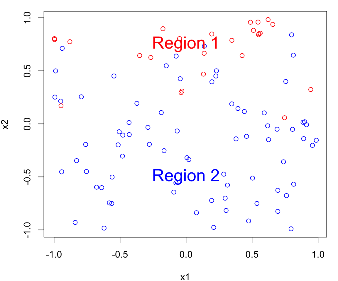
• Let’s simulate a data set with of two continuous predictors \(X_1\) and \(X_2\); both uniformly distributed from \([-1, 1]\).

• We create two classes:

  • a red group (corresponding to \(Y=0\)) and
  • a blue group (corresponding to \(Y=1\))

• To generate the class assignment we will only using \(X_2\).

• That is \(X_1\) is represents a useless predictor.

Class generation

We will assign an observation to a class based on the following:

If \(x_2 > 0\)

\[\begin{align} P(Y = 0 \mid X_2 = x_2) &= x_2\\ P(Y = 1 \mid X_2 = x_2) &= 1 - x_2 \end{align}\]

If \(x_2 \leq 0\)

\[\begin{align} P(Y = 0 \mid X_2 = x_2) &= 0\\ P(Y = 1 \mid X_2 = x_2) &= 1 \end{align}\]

Take the compliment of those probabilities to show the probabilities for belonging to the blue group:

Notice that \(x_{1i}\) does not provide any information about the class.

• The red and blue circles correspond to training observations that belong to two different classes.
• For each value of X1 and X2, there is a different probability of the response being red or blue.
• Since this is simulated data, we know how the data were generated and we can calculate the conditional probabilities for each value of X1 and X2.

• Any point above the dotted line reflects the set of points for which Pr(Y = red|X) is greater than 50%,
• while and point below the blue shaded region indicates the set of points for which the probability is below 50%.
• The purple dashed line represents the points where the probability is exactly 50%.

• The purple dashed line is called the Bayes decision boundary.
• The Bayes classifier’s prediction is determined by the Bayes decision boundary; an observation that falls on the red side of the boundary will be assigned to the red class, and similarly an observation on the blue side of the boundary will be assigned to the blue class.

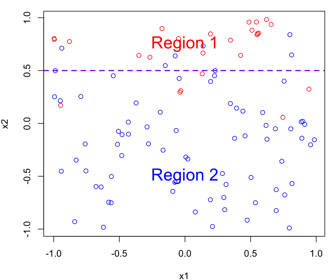
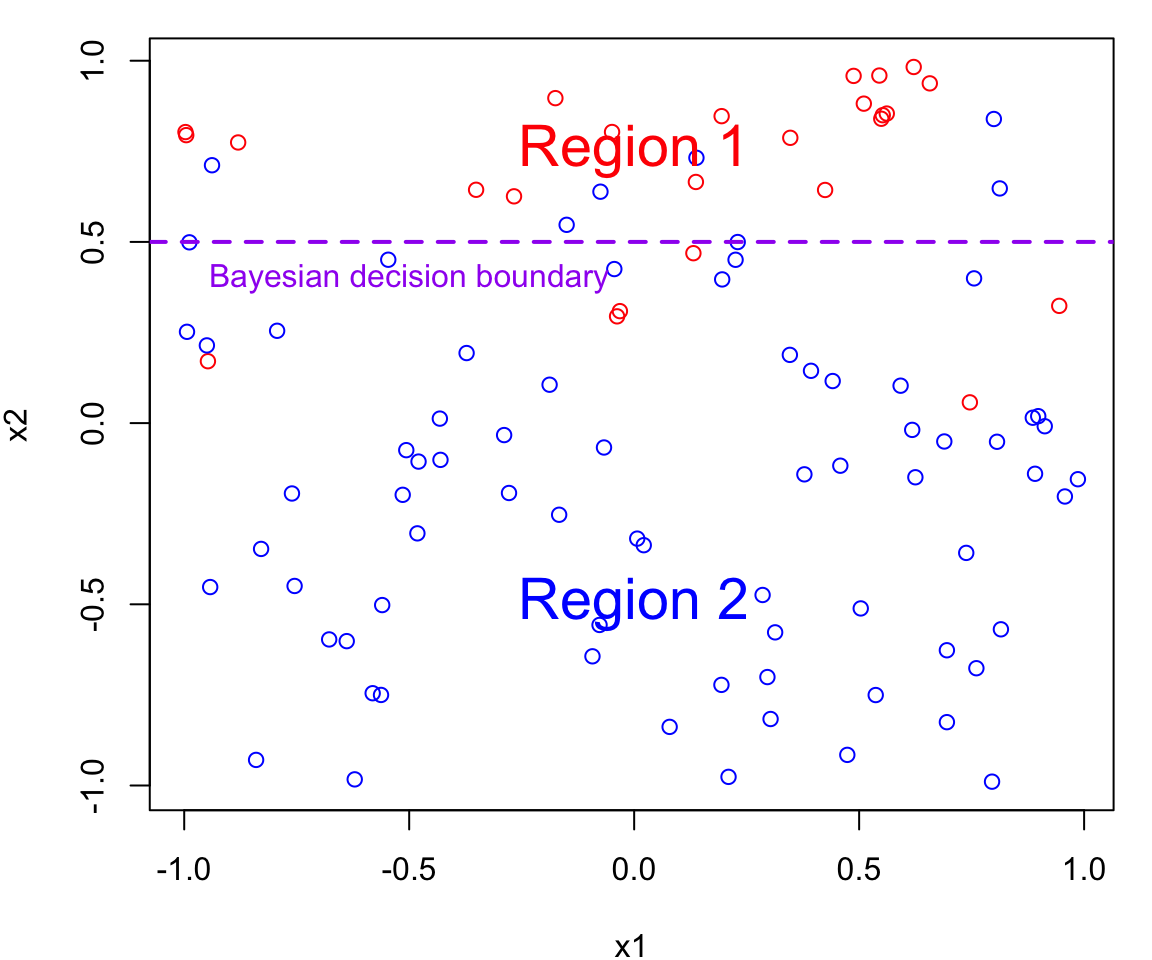
Bayes Decision Boundary

• The Bayes decision boundary represents the dividing line in the feature space (i.e. in terms of \(X\)s) that determines how data points are classified into different classes.

• In our case data points below the decision boundary (Region 1) are classified as red, while data points above the decision boundary (Region 2) are classified as blue

• Note that errors are still going to be made using this classifier since the process is random (points near the boundary are sometimes going to red in Region 2 and sometimes blue in Region 1)

heres its a line in higher dimension it can be a surface and we’ll see how it can take more complicated forms (eg. islands) later

Optimal Boundary

• The Bayes decision boundary represents the optimal decision boundary because it’s based on the true underlying probability distributions of the data.

• In other words, the Bayes decision boundary is going to make fewer mistakes than any other classifier you will come up with.

• However, in practice, these distributions are often unknown and need to be estimated from data, which can introduce uncertainty.

Bayes Error Rate

On average, Bayes classifier will yield the lowest possible test error rate given by the following expectation (averages the probability over all possible values of \(X\)) \[1-E\left( \max_j P(Y=j \mid X) \right)\]

The above is called the Bayes error rate which represents the minimum possible error rate that any classifier can achieve for a given classification problem.

• Our bayes error is greater than zero, because there is classes overlap in the true population so maxj Pr(Y = j|X = x0) < 1 for some values of \(x_0\).
• Notice if the is no error than the prob inside the () is 1 and the error is 0. But since there is some stochasic behaviour in our data Bayes error > 0
• You can think of this error as overlaping classes in your population 1 Problem: in practice we won’t know the conditional probability \(P(Y=j \mid X)\)!

The Bayes error rate is analogous to the irreducible error, discussed in previous lectures.

From simulations to real data

• In theory we would always like to predict qualitative responses using the Bayes classifier.
• But for real data, we do not know the conditional distribution of \(Y\) given \(X\), and so computing the Bayes classifier is impossible.
• Therefore, the Bayes classifier serves as an unattainable gold standard against which to compare other methods.

Classification Algorithms

• Many approaches attempt to estimate the conditional distribution of \(Y\) given \(X\), and then classify a given observation to the class with highest estimated probability.

• One example is the \(K\)-nearest neighbors (KNN) classifier.

• This algorithm is similar to the KNN regression, only now, rather than averaging continuous \(y\) values, we are counting the number of neighbors that belong to each class.

• The majority class among the \(K\)-nearest neighbors is chosen as the predicted class for the new data point.

KNN Classification

• Given a positive integer \(K\) and a test observation \(x_0\), the KNN classifier first identifies the \(K\) points in the training data that are closest to \(x_0\), represented by \(\mathcal{N}_0\).

• For each class \(j\), find \[\begin{equation} P(Y=j \mid X=x_0) \approx \frac{1}{K} \sum_{i \in N_0} I(y_i = j) \end{equation}\]

• Assign observation \(x_0\) to the class (\(j\)) for which the above probability is largest

Very intuitive, we look at the \(k\) closest values to a new point and see if they are mostly red or blue. Whichever class has the majority is the class where the object gets assigned

in R

To demo knn classification we will be using the knn function from the class package performs (other alternatives exist)

library("class")
knn(train, test, cl, k)

• train matrix or data frame of training set cases.
• test matrix or data frame of test set cases.
• cl factor of true classifications of training set
• k number of neighbours considered.

k - how to choose?

As indicated in the documentation “ties” are broken at random.

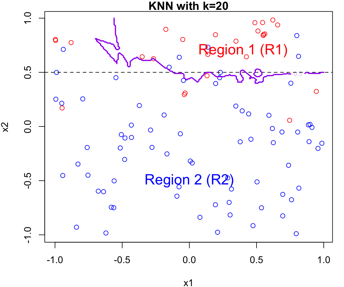
k Nearest Neighbours Example

• Let’s apply this algorithm to the simulated data considered previously.

• More specifically, we will fit knn for \(k = 20, 15, 9, 3\) and \(1\)

• Fair warning that the decision boundary and decision regions will not be as clear cut as our previous example.

• We will assess the error rate for each (code presented in lab)

An great interactive demo can be view here

So rather than a boundary like you get these little islands

Choosing k

• A key component of a “good” KNN classifier is determined by how we choose \(k\).

• \(k\) in a user-defined input to our algorithm which we can set anywhere from 1 to \(n\) (the number of points in our training set)

Question What would happen if \(k\) was set equal to \(n\)?

• every observation would get assigned to the most prevalent class in our training set.
• Since there are more red points than blue points, all future observations will get predicted to the red class.
• when \(k=n\) we predict the most common class (over simplistic)

Discuss some general rules of thumb for small/large \(k\)?

• Larger values of \(k\) tend to predict most commonly occurring class
• As \(k\) increase this model increase in simplicity and we get more BIAS
• As \(k\) decrease we tend to get overly flexible models, ie overfit. Boundaries change significantly with different training sets and the variance increases!
• What is this the product of? Bias-Variance tradeoff!
• You will see the same patter in the training (decreasing) and testing error (U shape); not shown here go to book.

Recap

Many approaches attempt to estimate the conditional distribution of \(Y\) given \(X\), and then classify a given observation to the class with highest estimated probability.

• KNN did this using a “voting” system with its nearest neighbours.

• Logistic regression uses the logistic function, e.g. \(P(Y = 1 \mid X = x) = \frac{e^{\beta_0 + \beta_1x}}{1 + e^{\beta_0 + \beta_1x}}\)

Let’s discuss linear and quadratic discriminant analysis as alternative methods for approximating the conditional distribution of \(Y\) given \(X\).

WHY logistic regression not natural in the MV setting

• When there is substantial separation between the two classes, the parameter estimates for the logistic regression model are surprisingly unstable. The methods that we consider in this section do not suffer from this problem.
• If the distribution of the predictors X is approximation normal in each class and the sample size is small this may be more accurate than Log reg

Discriminant Analysis

• Here the approach is to model the distribution of \(X\) in each of the classes separately, and then use Bayes’ theorem to flip things around and obtain \(\Pr(Y |X)\).
• When we use normal (Gaussian) distributions for each class, this leads to linear or quadratic discriminant analysis.
• However, this approach is quite general, and other distributions can be used as well. We will focus on normal distributions.

Generative Models for Classification

• Suppose we have qualitative response variable \(Y\) that can take on \(K\) possible distinct and unordered values.

• Suppose we have two groups, that is \(Y\) can take on two possible values \(K = 1, 2\) (corresponding to group 1/2)

• Let \(f_k(X) \equiv \Pr(X|Y = k)\) denote the density function of \(X\) for an observation that comes from the \(k\)th class.

• Let \(\pi_k\) represent the overall or prior probability that a randomly chosen observation comes from the \(k\)th class.

In other words, \(f_k(x)\) is relatively large if there is a high probability that an observation in the \(k\)th class has \(X \approx x\), and \(f_k(x)\) is small if it is very unlikely that an observation in the \(k\)th class has \(X \approx x\).

Applying Bayes Theorem

Then Bayes’ theorem states that

\[\begin{equation} \Pr(Y = k|X = x) = \frac{\pi_k f_k(x)}{\sum_{l=1}^{K} \pi_l f_l(x)} \end{equation}\]

This represents the posterior probability that an observation \(X = x\) belongs to the \(k\)th class.

• That is, it is the probability that the observation belongs to the kth class, given the predictor value for that observation.
• now let’s plug in the Gaussian distribution for \(f_k(x)\)

To estimate \(p_k(x)\), and thereby approximate the Bayes classifier, we can need to estimate the \(\pi_k\)s and \(f_k(x)\).

• estimating πk is easy if we have a random sample from the population: we simply compute the fraction of the training observations that belong to the kth class.
• However, estimating the density function fk(x) is much more challenging.
• As we will see, to estimate fk(x), we will typically have to make some simplifying assumptions.

We will abbreviate this to \(p_k(x) = \Pr(Y = k|X = x)\)

LDA for one predictor

• Let \(f(x ; \mu_k, \sigma_k)\) or \(f_k(x)\) be the probability density function (PDF) of an observation from the \(k\)th class.

• To estimate \(f_k(x)\), we will first make some assumptions about its form.

• The most commonly assumed PDF is the normal or Gaussian distribution with mean \(\mu\) and \(\sigma^2\) \[\begin{equation} f(x; \mu, \sigma) = \frac{1}{\sqrt{2\pi}\sigma} e^{-\frac{(x-\mu)^2}{2\sigma^2}} \end{equation}\]

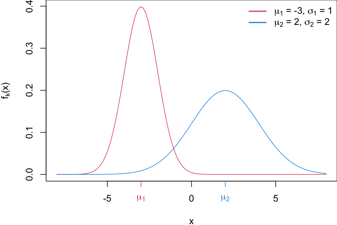
Univariate Normal Distribution

Sticking with univariate for now, suppose each group is normally distributed with different means and variances

\[\begin{align*} f_1(x) &\sim N(\mu_1, \sigma_1^2)\\ f_2(x) &\sim N(\mu_2, \sigma_2^2) \end{align*}\]

While discuss this method in 2-class univariate setting these concepts can be extended to the multivariate distributions with \(>2\) classes.

Plot of two univariate normals

Code

par(mar = c(3.9,4.1,0,0))
pi1 = 0.6
pi2 = 1 - pi1
curve(pi1*dnorm(x, mean = mean1, sd = sd1), col = 2, from = -8, 8, ylab = expression(paste(pi[k]*f[k]*"("* x *")")), lty = 2)
curve(pi2*dnorm(x, mean = mean2 , sd = sd2), col = 4, add = TRUE, lty = 2)
axis(1, at=mean1, labels = expression(mu[1]), col=2, col.axis=2)
axis(1, at=mean2, labels = expression(mu[2]), col=4, col.axis=4)        
gmm <- function(x, pis, mus, sigs){
  pis[1]*dnorm(x, mean = mus[1], sd = sigs[1]) +
    pis[2]*dnorm(x, mean = mus[2], sd = sigs[2]) 
}    
curve(gmm(x, c(pi1, pi2), c(mean1, mean2), c(sd1, sd2)), col = 3, add = TRUE)
ltext <- c(bquote(mu[1] *" = "* .(mean1)*", "*sigma[1] *" = "* .(sd1)),
           bquote(mu[2] *" = "* .(mean2)*", "*sigma[2] *" = "* .(sd2)),
           bquote(pi[1] *" = "* .(pi1)*", "*pi[2] *" = "* .(pi2)))
    legend("topright", lwd= 2, col = c(2,4, 3), 
           legend = ltext, bty = "n")

• we need to find the decision boundary
• We are going to classify a new point according to which numerator is the biggest

Building a classifier

We classify new points according to whichever numerator \((\pi_k f_k(x))\) is the highest.

Question: where would that decision boundary be on this picture?

• we need to find the decision boundary
• We are going to classify a new point according to which numerator is the biggest

LDA

• Linear Discriminant Analysis, or LDA for short, assumes that \(\sigma_1 = \sigma_2\)

• When we relax this assumption and allow for differing variances between groups, we get Quadratic Discriminant Analysis, or QDA for short

• For simplicity, we will focus on the LDA univariate case first with equal priors \(\pi_1 = \pi_2\)

• We will then focus on univariate LDA with equal priors \(\pi_1 = \pi_2\) and extend the ideas to multivariate QDA.

in other words, we assume there are the same number of training observations for both groups

If the class variances and priors are equal, the decision boundary is simply the average of the means

If the class variances and different and the priors are equal, the decision boundary is a function of sigma, the priors, and the means

• the boundary is where they intersect but it’s shifted to the right, which makes sense …
• there are more group 1 class than group 2 so the prior probability of belonging to class one is higher.
• the bigger prior has bumped up the rotted red curve and moved the decision boundary to the right
• there are more reds so all else being equal we are going to make less mistakes if we classify more observations to the red group.

LDA decision boundary

Since we’re dealing with two classes, we can set the decision boundary where \(p_1(x) = p_2(x)\)

\[\begin{align} \frac{\pi_1 f_1(x)}{\sum_{l=1}^{K} \pi_l f_l(x)} &= \frac{\pi_2 f_2(x)}{\sum_{l=1}^{K} \pi_l f_l(x)} \\ \frac{\pi_1}{\sqrt{2\pi}\sigma} e^{-\frac{(x-\mu_1)^2}{2\sigma^2}} &= \frac{\pi_2}{\sqrt{2\pi}\sigma} e^{-\frac{(x-\mu_2)^2}{2\sigma^2}}\\ \vdots \end{align}\]

denoms are common

Discriminant score

This is boils down to to assigning the observation to the class for which discriminant score \(\delta_k(x)\) is the largest: \[\begin{equation} \delta_k(x) = x \cdot \frac{\mu_k}{\sigma^2} - \frac{\mu_{k}^2}{\sigma^2} + \log(\pi_k) \end{equation}\]

notice it involes x, the mean and variance and priors

Decision boundary

The Bayes decision boundary when \(\pi_1 = \pi_2\) is found at: \[\begin{equation} x = \frac{\mu_1^2 - \mu_2^2}{2(\mu_1 - \mu_2)} = \frac{\mu_1 + \mu_2}{2} \end{equation}\]

Let’s find the Bayes decision boundary when \(\pi_1 \neq \pi_2\) …

leave to show for the assignment

Taking the log of both sides and rearranging the terms, it is not hard to show that this is equivalent to assigning the observation to the class for which

that is there is a shared variance term across all classes

1. Bayes Theorem

2. \(\pi_k\) = Prior probability X comes from the $k$th class.

• easy to estimate (prop of obs belonging to the $k$th class or using prior knowledge of the class membership probabilities directly.)

3. Est parameters of \(f_k(x)\) trickier (have to make some simplifying assumptions)

This is boils down to to assigning the observation to the class for which \(\delta_k(x)\) is the largest: \[\begin{equation} \delta_k(x) = x \cdot \mu_k - \mu_{2k} + \log(\pi_k) \end{equation}\]

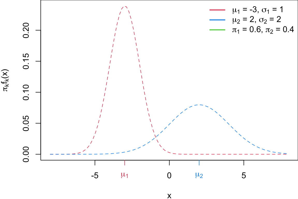
Probability of each class

Where \(\pi_1\) = 0.8, \(\pi_2\) = 0.2, \(\sigma = \sigma_1 = \sigma_2\) = 2, \(\mu_1\) = -3 \(\mu_2\) = 2 and x = 0.61

Code

gmm <- function(x, pis, mus, sigs){
  pis[1]*dnorm(x, mean = mus[1], sd = sigs[1]) +
    pis[2]*dnorm(x, mean = mus[2], sd = sigs[2]) 
}    
denom = gmm(x,c(pi1,pi2), c(mean1, mean2), c(sd1, sd2))

Code

# Pr(y = 1 | x )
pi1*dnorm(x, mean1, sd1)/denom

[1] 0.4996986

\[ \begin{align} P(&Y = 1 \mid x = 0.61) \\ &= \frac{\pi_1 f_1(x)}{\pi_1 f_1(x) + \pi_2 f_2(x)}\\ &= \frac{0.8 \cdot 0.04} {0.8 \cdot 0.04 + 0.2 \cdot 0.16}\\ &= 0.5 \end{align} \]

Code

# Pr(y = 2 | x )
pi2*dnorm(x, mean2, sd2)/denom

[1] 0.5003014

\[ \begin{align} P(&Y = 2 \mid x = 0.61) \\ &= \frac{\pi_2 f_2(x)}{\pi_1 f_1(x) + \pi_2 f_2(x)}\\ &= \frac{0.2 \cdot 0.16} {0.8 \cdot 0.04 + 0.2 \cdot 0.16}\\ &= 0.5 \end{align} \]

Why discriminant analysis

• If \(n\) is small and the distribution of the predictors \(X\) is approximately normal in each of the classes, the linear discriminant model is more stable than the logistic regression model.
• When the classes are well-separated, the parameter estimates for the logistic regression model are surprisingly unstable. Linear discriminant analysis does not suffer from this problem.
• LDA is popular when we have more than two response classes, because it also provides low-dimensional views of the data (we’ll return to this idea later)

• if you look up LDA you might here it being explained more along the lines of PCA (e.g. statquest)
• we will get back to this point when we talk about PCA (to which LDA has some similarities)
• Both LDA and PCA can be used as for dimensionality reduction Rob’s final note:
• when we’ve specified the correct population model (i.e. if our normal assumption is right) this is the best we’re going to be able to do.
  

Classifier

When we do not have equal variance (i.e \(sigma_1 \neq \sigma_2\)) our classifier predicts \(x_0\) to group 1 if

\[ \pi_1 \cdot f_1(x; \mu_1, \sigma_1) > \pi_2\cdot f_2(x; \mu_2, \sigma_2) \]

More generally, we classify observation \(x\) based on the following rule:

\[ \hat y = \underset{k}{\operatorname{argmax}} \pi_k \cdot f_k(x; \mu_k, \sigma_k) \]

above I was using dnorm() function to calculate this, but what do we do now?

But we don’t know \(f_k\)

No problem. We estimate them!

ILSR2 Figure 4.4: Left: Two one-dimensional normal density functions are shown. The dashed vertical line represents the Bayes decision boundary. Right: 20 observations were drawn from each of the two classes, and are shown as histograms. The Bayes decision boundary is again shown as a dashed vertical line. The solid vertical line represents the LDA decision boundary estimated from the training data.

Parameter Estimates

\[\begin{align} \hat{\pi}_k &= \frac{n_k}{n} \quad\quad \hat{\mu}_k = \frac{1}{n_k} \sum_{i: y_i=k} x_i\\ \hat{\sigma}^2 &= \frac{1}{n - K} \sum_{k=1}^{K} \sum_{i: y_i=k} (x_i - \hat{\mu}_k)^2 \end{align}\]

where \(n\) is the total number of training observations, \(n_k\) is the number of observations in class \(k\), and \(\mu_k\) and \(\hat{\sigma}^2_k\) are the MLE estimates for mean and (pooled) variance in the \(k\)th class.

• estimated priors are obvious: the number of obs in each class divided by the total number of observations
• means = sample mean
• the pooled variance is just a weighted average of the sample variances
• so plugging those estimates into the formula we get an estimate for the decision boundary

\(\sum_{i: y_i=k}\) represents a sum over all values of \(i\) for which the condition \(y_i=k\) holds true

Multivariate Normal Distribution

For Discriminant analysis when \(p>1\) we use the Multivariate Normal Distribution (MVN).

A MVN random vector \(\mathbf X\), has probability distribution given by \[f(\mathbf x) = \frac{1}{(2\pi)^{p/2}|\boldsymbol{\Sigma}|^{1/2}} e^{-\frac{1}{2}(\mathbf{x}-\boldsymbol{\mu})^T\boldsymbol{\Sigma}^{-1}(\mathbf{x}-\boldsymbol{\mu})}\] with mean vector \(\boldsymbol{\mu}\) and covariance matrix \(\boldsymbol{\Sigma}\).

• covariance is a measure of the joint probability to two random variables.

• value difficult to interpret because it depends on scale (normalized version = correlation)

To indicate that a \(p\)-dimensional random variable \(X\) has a multivariate Gaussian distribution, we write \(\mathbf X \sim \mathcal{N}(\boldsymbol\mu, \boldsymbol\Sigma)\).

3D Plot of Multivariate Normal

Source: Wikipedia (Multivariate Normal Distribution)

• These are two common classification algorithms that you’ll run into.

• The only different in LDA vs QDA is there assumption on \(\Sigma\)

• we can relax the assumption of \(\pi_k\)s and they will still both have a linear and quadratic boundary.

Covariance Matrix

• The covariance matrix is symmetric a square matrix where each entry \(\Sigma_{ij}\) represents the covariance between variables \(X_i\) and \(X_j\)

• The diagonal elements (\(\sigma_{i}\)) represent the variances of individual variables, and the off-diagonal elements (\(\sigma_{ij}\) for \(i\neq j\)) represent the covariances between pairs of variables. \[\begin{equation} \boldsymbol \Sigma = \begin{bmatrix} \sigma_{1}^2 & \sigma_{12} & \ldots & \sigma_{1p} \\ \sigma_{12} & \sigma_{2}^2 & \ldots & \sigma_{2p} \\ \vdots & \vdots & \ddots & \vdots \\ \sigma_{1p} & \sigma_{2p} & \ldots & \sigma_{p}^2 \end{bmatrix} \quad \text{ where }\sigma_{ij} = \sigma_{ji} = \text{Cov}(X_i, X_j) \end{equation}\]

Recall the relationship between correlation (\(r\)) and covariance for two random variables \(X\) and \(Y\): \(r = \frac{\text{Cov}(X,Y)}{\sigma_X \cdot \sigma_Y}\)

Uncorrelated

Code

# Install and load the required libraries
library(plotly)
library(mvtnorm)

# Parameters for the multivariate normal distribution
mean_vec <- c(0, 0)  # Mean vector
cov_mat <- matrix(c(1, 0, 0, 1), nrow = 2)  # Covariance matrix

# Generate data grid
x <- seq(-3, 3, length.out = 100)
y <- seq(-3, 3, length.out = 100)
grid <- expand.grid(x, y)

# Calculate the multivariate normal density for each point in the grid
z <- dmvnorm(grid, mean = mean_vec, sigma = cov_mat)

# Reshape the z values to match the grid dimensions
z_matrix <- matrix(z, nrow = length(x), ncol = length(y))

# Create an interactive 3D surface plot using plotly
plot_ly(z = ~z_matrix, x = ~x, y = ~y, type = "surface") %>%
  layout(scene = list(
    xaxis = list(title = "X-axis"),
    yaxis = list(title = "Y-axis"),
    zaxis = list(title = "Density")
  ))

uncorrelated - like a symetric bell/cone

Code

# Install and load the required libraries
library(plotly)
library(mvtnorm)

# Parameters for the multivariate normal distribution
mean_vec <- c(0, 0)  # Mean vector
cov_mat <- matrix(c(1, 0.5, 0.5, 1), nrow = 2)  # Covariance matrix

# Generate data grid
x <- seq(-3, 3, length.out = 100)
y <- seq(-3, 3, length.out = 100)
grid <- expand.grid(x, y)

# Calculate the multivariate normal density for each point in the grid
z <- dmvnorm(grid, mean = mean_vec, sigma = cov_mat)

# Reshape the z values to match the grid dimensions
z_matrix <- matrix(z, nrow = length(x), ncol = length(y))

# Create an interactive 3D surface plot using plotly
plot_ly(z = ~z_matrix, x = ~x, y = ~y, type = "surface") %>%
  layout(scene = list(
    xaxis = list(title = "X-axis"),
    yaxis = list(title = "Y-axis"),
    zaxis = list(title = "Density")
  ))

correlated - We get stretches in certain directions

LDA when \(p>1\)

• In the case of \(p > 1\) predictors, the LDA classifier assumes that the observations in the \(k\)th class are drawn from a multivariate Gaussian distribution \(\mathcal{N}(\boldsymbol\mu_k, \boldsymbol\Sigma)\), where \(\boldsymbol\mu_k\) is a class-specific mean vector, and \(\boldsymbol\Sigma\) is a covariance matrix that is common to all \(K\) classes.

• Algebra reveals that the Bayes classifier assigns an observation \(X = x\) to the class for which \[\begin{equation} \delta_k(x) = x^T \boldsymbol\Sigma^{-1} \boldsymbol\mu_k - \frac{1}{2} \boldsymbol\mu_k^T \boldsymbol\Sigma^{-1} \boldsymbol\mu_k + \log(\pi_k) \end{equation}\]

this is the linear function

What does equal Covariance look like?

Source of image [1]

Contour Plots (equal covariance)

Code

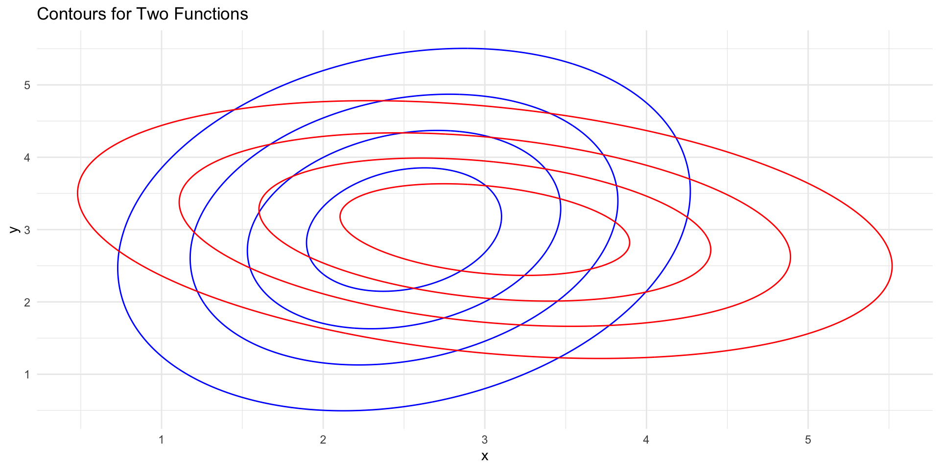
# Load the required libraries
library(ggplot2)
library(mvtnorm)
library(cowplot)

# Set a random seed for reproducibility
set.seed(123)

# Define the means and covariance matrix
mean1 <- c(2, 3)  # Mean vector for distribution 1
mean2 <- c(4, 4)  # Mean vector for distribution 2
cov_matrix <- matrix(c(1, 0.5, 0.5, 1), nrow = 2)  # Shared covariance matrix

# Generate data grid
x <- seq(0, 6, length.out = 400)
y <- seq(0.5, 6.5, length.out = 400)
grid <- expand.grid(x, y)

# Calculate the density for each point in the grid for both distributions
z1 <- dmvnorm(grid, mean = mean1, sigma = cov_matrix)
z2 <- dmvnorm(grid, mean = mean2, sigma = cov_matrix)


# Combine the densities into a data frame
data1 <- data.frame(x = rep(x, length(y)), y = rep(y, each = length(x)), z = z1)
data2 <- data.frame(x = rep(x, length(y)), y = rep(y, each = length(x)), z = z2)


 ggplot() +
  geom_contour(data = data1, aes(x = x, y = y, z = z), color = "blue", bins = 8) +
  geom_contour(data = data2, aes(x = x, y = y, z = z), color = "red", bins = 8) +
  labs(title = "Contours for Two Functions") +
  theme_minimal()

Illustration \(p = 2\) and \(K=3\)

ILSR Fig 4.6: Here \(\pi_1 = \pi_2 = \pi_3\) Left: Ellipses that contain 95 % of the probability for each of the three classes are shown. The dashed lines are the Bayes decision boundaries. Right: 20 observations were generated from each class, and the corresponding LDA decision boundaries are indicated using solid black lines. The Bayes decision boundaries are shown as dashed lines.

• equal pis imply same number of training set values

• devision boundardies corresponds to where the contours intersect

• if the bayes decision boundaries were know, they would yeild the fewest mislassification errors, amoung all possilbe classifers

LDA to QDA

• When \(f_k(x)\) are Gaussian densities, with the same covariance matrix \(\boldsymbol\Sigma\) in each class, this leads to linear discriminant analysis.

• With Gaussians but different \(\boldsymbol \Sigma_k\) in each class, we get quadratic discriminant analysis.

• Because the \(\boldsymbol\Sigma_k\) are different, we don’t loose the quadratic terms so we get discriminant function is now

\[\begin{equation} \delta_k(x) = -\frac{1}{2}(x - \mu_k)^T \boldsymbol \Sigma_k^{-1} (x - \mu_k) + \log \pi_k - \frac{1}{2} \log |\Sigma_k| \end{equation}\]

• By altering the forms for (f_k(x)), we get different classifiers.

where \(|\Sigma_k|\) is the determinant of the covariance matrix

Contour Plots (unequal covariance)

Code

# Load the required libraries
library(ggplot2)
library(mvtnorm)
library(cowplot)

# Set a random seed for reproducibility
set.seed(123)

# Define the means and covariance matrix
mean1 <- c(2.5, 3)
mean2 <- c(3, 3)

# Define different covariance matrices for the two distributions
cov_matrix1 <- matrix(c(1, 0.3, 0.3, 2), nrow = 2)
cov_matrix2 <- matrix(c(2, -0.4, -0.4, 1), nrow = 2)

# Generate data grid
x <- seq(-1, 6, length.out = 400)
y <- seq(-1, 6.5, length.out = 400)
grid <- expand.grid(x, y)

# Calculate the density for each point in the grid for both distributions
z1 <- dmvnorm(grid, mean = mean1, sigma = cov_matrix1)
z2 <- dmvnorm(grid, mean = mean2, sigma = cov_matrix2)


# Combine the densities into a data frame
data1 <- data.frame(x = rep(x, length(y)), y = rep(y, each = length(x)), z = z1)
data2 <- data.frame(x = rep(x, length(y)), y = rep(y, each = length(x)), z = z2)


 ggplot() +
  geom_contour(data = data1, aes(x = x, y = y, z = z), color = "blue", bins = 5) +
  geom_contour(data = data2, aes(x = x, y = y, z = z), color = "red", bins = 5) +
  labs(title = "Contours for Two Functions") +
  theme_minimal()

Summary

Both LDA and QDA assumes each class follows an underlying Gaussian distribution

LDA

• assumes equal variance across classes

• PRO: easier to fit

• CON: less flexible

QDA

• doesn’t assume equal variance across classes

• PRO: often leads to a lower error rate

• CON: reduced intelligibility

Bias-variance tradeoff: the LDA can be too simple whereas the QDA has a higher risk of overfitting to our data.

Example: Iris

4 variables 3 species 50 samples/class:

• Setosa (blue)
• Versicolor (green)
• Virginica (orange)

Code

par(mar = c(3.9, 3.9, 0, 1))        # reduce even more 
lookup <- c(setosa='blue', versicola='green', virginica='orange')
col.ind <- lookup[iris$Species]
pairs(iris[-5], pch=21, col="gray", bg=col.ind)

LDA fitted model

Let’s fit the LDA classifier using all 4 predictors

lda.fit <- lda(Species ~ ., data = iris)
lda.fit

...
Prior probabilities of groups:
    setosa versicolor  virginica 
 0.3333333  0.3333333  0.3333333 

Group means:
           Sepal.Length Sepal.Width Petal.Length Petal.Width
setosa            5.006       3.428        1.462       0.246
versicolor        5.936       2.770        4.260       1.326
virginica         6.588       2.974        5.552       2.026

...

• The output shows that the prior probabilities of each group (setosa, versicolor, and virginica) are all equal at 0.33.
• The group means section shows the mean values of each input variable (sepal length, sepal width, petal length, and petal width) for each group.

coefficients of linear discriminants: are the weights of the linear combination of the input variables that best separates the groups. - The “LD1” and “LD2” columns represent the first and second linear discriminant functions, respectively. - Each row represents the weight of a particular input variable in the linear combination.

the proportion of trace is the proportion of the total variability in the input variables that is explained by each linear discriminant function. - the first linear discriminant function (LD1) explains 99.12% of the total variability, - the second linear discriminant function (LD2) explains only 0.88%. This indicates that most of the discriminatory power of the input variables is captured by the first linear discriminant function.

Plotted fit

plot(Sepal.Width ~ Sepal.Length, data = iris, pch=21, col="gray", bg= col.ind)
points(lda.fit$means[,1], lda.fit$means[,2], pch=21, cex=2,
       col="black", bg=lookup)

This of course is the training error so it may be overly optimistic.

Classification Table

LDA classifies all but 3 of the 150 training samples correctly.

lda.pred <- predict(lda.fit) # this is a list
names(lda.pred)

[1] "class"     "posterior" "x"        

table(iris$Species, lda.pred$class)

            
             setosa versicolor virginica
  setosa         50          0         0
  versicolor      0         48         2
  virginica       0          1        49

From \(\delta_k(x)\) to probabilities

From \(\delta_k(x)\) to probabilities, once we have estimates \(\hat{\delta}_k(x)\), we can turn these into estimates for class probabilities:

\[\begin{align} \Pr(Y = k \,|\, X = x) = \frac{e^{\hat{\delta}_k(x)}}{\sum_{l=1}^{K} e^{\hat{\delta}_l(x)}} \end{align}\]

So classifying to the largest \(\hat{\delta}_k(x)\) amounts to classifying to the class for which \(\Pr(Y = k \,|\, X = x)\) is largest.

• it’s not that hard to show
• we can actually look at methods where we change that thershold to 0.8 instead of 0.5

Like in logisitic regression, for \(K = 2\), we classify to class 2 if \(\Pr(Y = 2 \,|\, X = x) \geq 0.5\) else to class 1.