Lab Tutorial 7

Summary: This lab focuses on Simple Regression Analysis using KNN.

Towards the end of the lab, you will find a set of assignment exercises (Assignment 6). These assignments are to be completed and submitted on Canvas.

Lab 07

After completing this week’s lecture and tutorial work, you will be able to:

• Recognize situations where a simple regression analysis would be appropriate for making predictions.

• Explain the k-nearest neighbour (\(k\)-nn) regression algorithm and describe how it differs from \(k\)-nn classification.

• Interpret the output of a \(k\)-nn regression.

• In a dataset with two variables, perform k-nearest neighbour regression in R using tidymodels to predict the values for a test dataset.

• Using R, execute cross-validation in R to choose the number of neighbours.

• Using R, evaluate \(k\)-nn regression prediction accuracy using a test data set and an appropriate metric (e.g., root mean square prediction error, RMSPE).

• In the context of \(k\)-nn regression, compare and contrast goodness of fit and prediction properties (namely RMSE vs RMSPE).

• Describe advantages and disadvantages of the \(k\)-nearest neighbour regression approach.

### Run this cell before continuing. 
library(tidyverse)
library(repr)
library(tidymodels)
options(repr.matrix.max.rows = 6)

Marathon Training

Source: https://media.giphy.com/media/nUN6InE2CodRm/giphy.gif

What predicts which athletes will perform better than others? Specifically, we are interested in marathon runners, and looking at how the maximum distance ran per week (in miles) during race training predicts the time it takes a runner to finish the race? For this, we will be looking at the marathon.csv file that can be downloaded from Datasets module on course Canvas. Save the file in your data/ folder.

First, load the data and assign it to an object called marathon.

Click for answer

marathon <- read_csv("../data/marathon.csv")

Rows: 929 Columns: 13
── Column specification ────────────────────────────────────────────────────────
Delimiter: ","
dbl (13): age, bmi, female, footwear, group, injury, mf_d, mf_di, mf_ti, max...

ℹ Use `spec()` to retrieve the full column specification for this data.
ℹ Specify the column types or set `show_col_types = FALSE` to quiet this message.

Click for answer

#or
#marathon <- read_csv("data/marathon.csv")

We want to predict race time (in hours) (time_hrs) given a particular value of maximum distance ran per week (in miles) during race training (max).

Let’s take a subset of size 50 individuals of our marathon data and assign it to an object called marathon_50. With this subset, plot a scatterplot to assess the relationship between these two variables. Put time_hrs on the y-axis and max on the x-axis. Assign this plot to an object called answer1. What’s the relationship between race time and maximum distance ran per week during training based on the scatterplot you create below.

Hint: To take a subset of your data you can use the slice_sample() function

options(repr.plot.width = 8, repr.plot.height = 7)

set.seed(2000) ### DO NOT CHANGE

#... <- ... |>
#    slice_sample(...)

# your code here

Click for answer

options(repr.plot.width = 8, repr.plot.height = 7)

set.seed(2000) ### DO NOT CHANGE

marathon_50<- marathon |> slice_sample(n = 50)

answer1 <- ggplot(marathon_50, aes(x = max, y = time_hrs)) +
  geom_point(alpha = 0.4) +
  xlab("Maximum Distance Ran per \n Week During Training (mi)") +
  ylab("Race Time (hours)") + 
  theme(text = element_text(size = 12))
answer1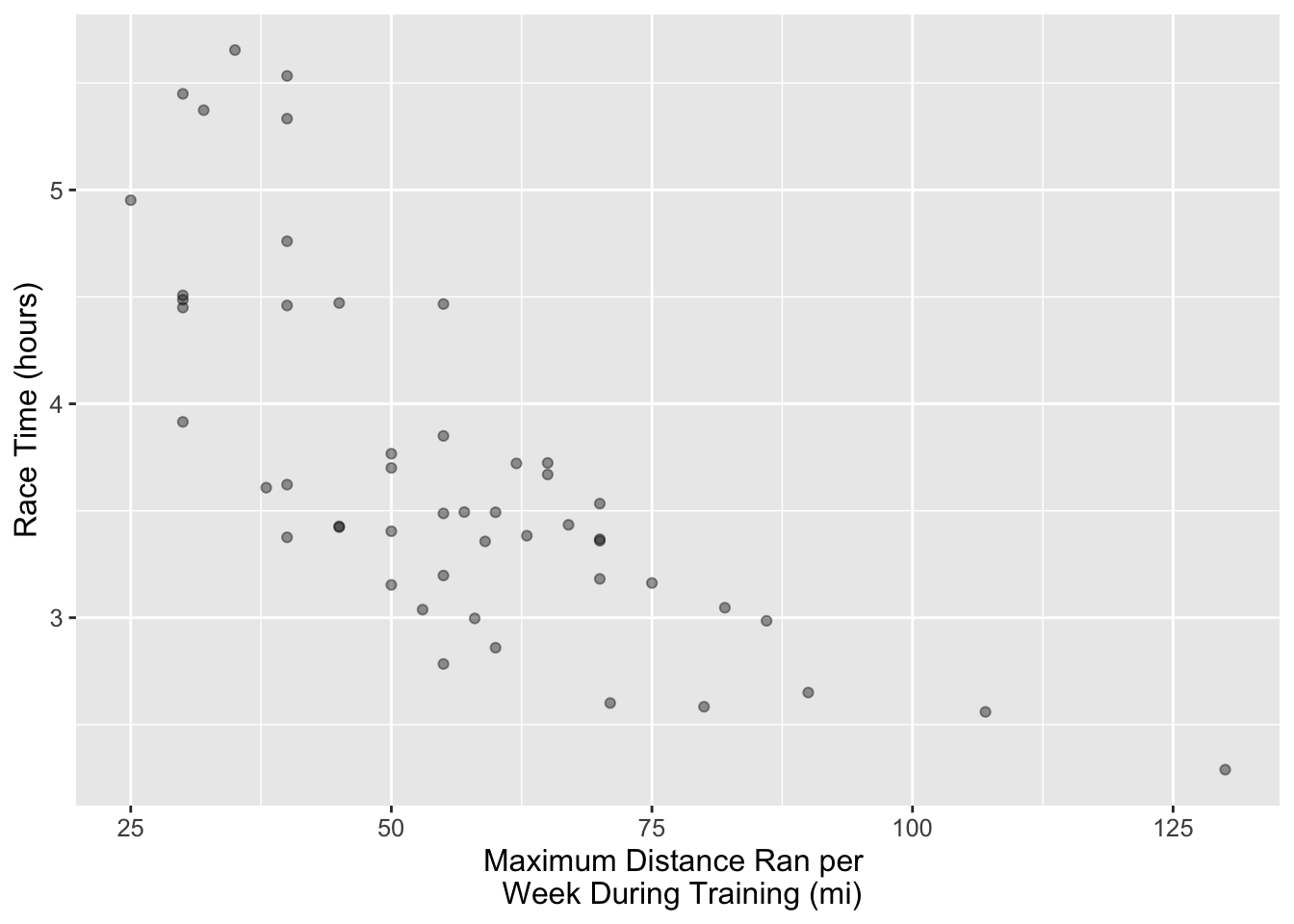

Click for answer

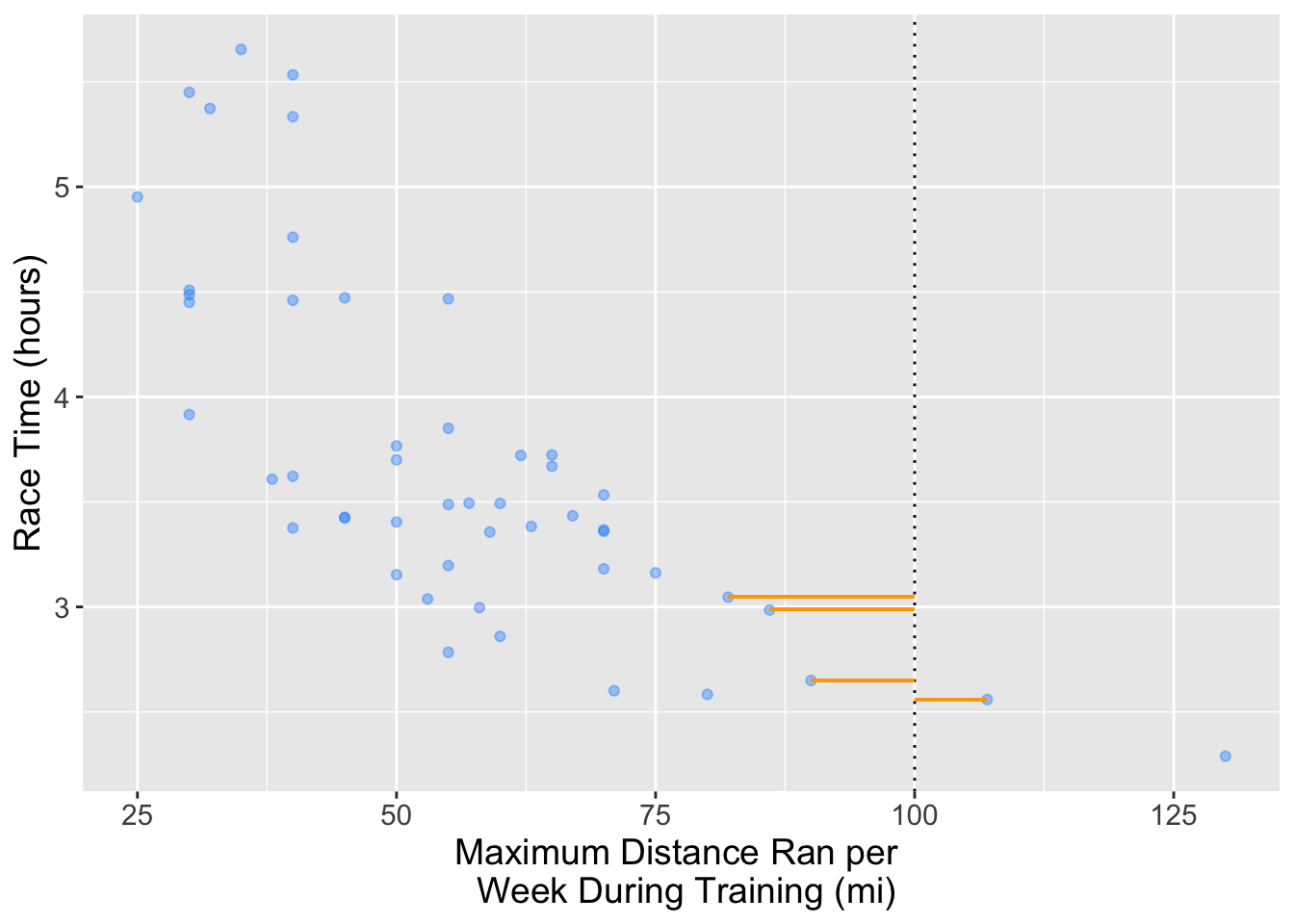
# According to the scatter plot, there is a negative correlation between these two variables, indicating that, on average, as race time increases, the maximum weekly distance run decreases.

Suppose we want to predict the race time for someone who ran a maximum distance of 100 miles per week during training. In the plot below we can see that no one has run a maximum distance of 100 miles per week. But, if we are interested in prediction, how can we predict with this data? We can use \(k\)-nn regression! To do this we get the \(Y\) values (target/response variable) of the nearest \(k\) values and then take their average and use that as the prediction.

For this question predict the race time based on the 4 closest neighbors to the 100 miles per week during training.

Fill in the scaffolding below and assign your answer to an object named answer2.

#... <- ... |> 
#  mutate(diff = abs(100 - ...)) |> 
#  ...(diff, ...) |> 
#  summarise(predicted = ...(...)) |>
#  pull()

# your code here

Click for answer

answer2 <- marathon_50 |> 
  mutate(diff = abs(100 - max)) |>
  slice_min(diff, n = 4) |> 
  summarise(predicted = mean(time_hrs)) |>
  pull()
answer2

[1] 2.810347

This time, let’s instead predict the race time based on the 2 closest neighbors to the 100 miles per week during training.

Assign your answer to an object named answer3.

Click for answer

answer3 <- marathon_50 |> 
  mutate(diff = abs(100 - max)) |>
  slice_min(diff, n = 2) |> 
  summarise(predicted = mean(time_hrs)) |>
  pull()

answer3

[1] 2.604722

So far you have calculated the \(k\) nearest neighbors predictions manually based on \(k\)’s we have told you to use. However, last week we learned how to use a better method to choose the best \(k\) for classification.

Based on what you learned last week and what you have learned about \(k\)-nn regression so far this week, which method would you use to choose the \(k\) (in the situation where we don’t tell you which \(k\) to use)?

• 1. Choose the \(k\) that excludes most outliers
• 2. Choose the \(k\) with the lowest training error
• 3. Choose the \(k\) with the lowest cross-validation error
• 4. Choose the \(k\) that includes the most data points
• 5. Choose the \(k\) with the lowest testing error

Click for answer

# C

We have just seen how to perform k-nn regression manually, now we will apply it to the whole dataset using the tidymodels package. To do so, we will first need to create the training and testing datasets. Split the data using 75% of the marathon data as your training set and set time_hrs as the strata argument. Store this data into an object called marathon_split.

Then, use the appropriate training and testing functions to create your training set which you will call marathon_training and your testing set which you will call marathon_testing. Remember we won’t touch the test dataset until the end.

set.seed(2000) ### DO NOT CHANGE

#... <- initial_split(..., prop = ..., strata = ...)
#... <- training(...)
#... <- testing(...)

Click for answer

set.seed(2000)
marathon_split <- initial_split(marathon, prop = 0.75, strata = time_hrs)
marathon_training<- training(marathon_split)
marathon_testing<- testing(marathon_split)

Next, we’ll use cross-validation on our training data to choose \(k\). In \(k\)-nn classification, we used accuracy to see how well our predictions matched the true labels. In the context of \(k\)-nn regression, we will use RMPSE instead. Interpreting the RMPSE value can be tricky but generally speaking, if the prediction values are very close to the true values, the RMSPE will be small. Conversely, if the prediction values are not very close to the true values, the RMSPE will be quite large.

Let’s perform a cross-validation and choose the optimal \(k\). First, create a model specification for \(k\)-nn. We are still using the \(k\)-nearest neighbours algorithm, and so we will still use the same package for the model engine as we did in classification ("kknn"). As usual, specify that we want to use the straight-line distance. However, since this will be a regression problem, we will use set_mode("regression") in the model specification. Store your model specification in an object called marathon_spec.

Moreover, create a recipe to preprocess our data. Store your recipe in an object called marathon_recipe. The recipe should specify that the response variable is race time (hrs) and the predictor is maximum distance ran per week during training.

set.seed(1234) #DO NOT REMOVE

#... <- nearest_neighbor(weight_func = ..., neighbors = ...) |> 
#       set_engine(...) |>
#       set_mode(...) 

#... <- recipe(... ~ ..., data = ...) |>
#       step_scale(...) |>
#       step_center(...)
#  

Click for answer

set.seed(1234) 

marathon_spec <- nearest_neighbor(weight_func = "rectangular", 
                                  neighbors = tune()) |>
  set_engine("kknn") |>
  set_mode("regression")

marathon_recipe<- recipe(time_hrs ~ max , data = marathon_training) |>
  step_scale(all_predictors()) |>
  step_center(all_predictors())

Now, create the splits for cross-validation with 5 folds using the vfold_cv function. Store your answer in an object called marathon_vfold. Make sure to set the strata argument.

Then, use the workflow function to combine your model specification and recipe. Store your answer in an object called marathon_workflow.

Click for answer

set.seed(1234)
marathon_vfold <- vfold_cv(marathon_training, v = 5, strata = time_hrs)
marathon_workflow <- workflow() |>
  add_recipe(marathon_recipe) |>
  add_model(marathon_spec)

marathon_workflow

══ Workflow ════════════════════════════════════════════════════════════════════
Preprocessor: Recipe
Model: nearest_neighbor()

── Preprocessor ────────────────────────────────────────────────────────────────
2 Recipe Steps

• step_scale()
• step_center()

── Model ───────────────────────────────────────────────────────────────────────
K-Nearest Neighbor Model Specification (regression)

Main Arguments:
  neighbors = tune()
  weight_func = rectangular

Computational engine: kknn 

If you haven’t noticed by now, the major difference compared to other workflows from prevous lectures is that we are running a regression rather than a classification. Specifying regression in the set_mode function essentially tells tidymodels that we need to use different metrics (RMPSE rather than accuracy) for tuning and evaluation.

Now, let’s use the RMSPE to find the best setting for \(k\) from our workflow. Let’s test the values \(k = 1, 11, 21, 31, ..., 81\).

First, create a tibble with a column called neighbors that contains the sequence of values. Remember that you should use the seq function to create the range of \(k\)s that goes from 1 to 81 by jumps of 10. Assign that tibble to an object called gridvals.

Next, tune your workflow such that it tests all the values in gridvals and resamples using your cross-validation data set. Finally, collect the statistics from your model. Assign your answer to an object called marathon_results.

Click for answer

gridvals <- tibble(neighbors = seq(from = 1, to = 81, by = 10))

marathon_results <- marathon_workflow |>
  tune_grid(resamples = marathon_vfold, grid = gridvals) |>
  collect_metrics() |>
  filter(.metric == "rmse")

marathon_results

# A tibble: 9 × 7
  neighbors .metric .estimator  mean     n std_err .config             
      <dbl> <chr>   <chr>      <dbl> <int>   <dbl> <chr>               
1         1 rmse    standard   0.963     5  0.0382 Preprocessor1_Model1
2        11 rmse    standard   0.730     5  0.0322 Preprocessor1_Model2
3        21 rmse    standard   0.654     5  0.0295 Preprocessor1_Model3
4        31 rmse    standard   0.629     5  0.0257 Preprocessor1_Model4
5        41 rmse    standard   0.611     5  0.0194 Preprocessor1_Model5
6        51 rmse    standard   0.602     5  0.0151 Preprocessor1_Model6
7        61 rmse    standard   0.599     5  0.0150 Preprocessor1_Model7
8        71 rmse    standard   0.597     5  0.0151 Preprocessor1_Model8
9        81 rmse    standard   0.598     5  0.0158 Preprocessor1_Model9

Great! Now find the minimum RMSPE along with it’s associated metrics such as the mean and standard error, to help us find the number of neighbors that will serve as our best \(k\) value. Your answer should simply be a tibble with one row. Assign your answer to an object called marathon_min.

set.seed(2020) # DO NOT REMOVE

#... <- marathon_results |>
#    filter(... == min(...))

Click for answer

set.seed(2020) 

marathon_min <- marathon_results |>
  filter(mean == min(mean))
marathon_min

# A tibble: 1 × 7
  neighbors .metric .estimator  mean     n std_err .config             
      <dbl> <chr>   <chr>      <dbl> <int>   <dbl> <chr>               
1        71 rmse    standard   0.597     5  0.0151 Preprocessor1_Model8

To assess how well our model might do at predicting on unseen data, we will assess its RMSPE on the test data. To do this, we will first re-train our \(k\)-nn regression model on the entire training data set, using the \(K\) value we obtained from prevous question.

To start, pull the best neighbors value from marathon_min and store it an object called k_min.

Following that, we will repeat the workflow analysis again but with a brand new model specification with k_min. Remember, we are doing a regression analysis, so please select the appropriate mode. Store your new model specification in an object called marathon_best_spec and your new workflow analysis in an object called marathon_best_fit. You can reuse this marathon_recipe for this workflow, as we do not need to change it for this task.

Then, we will use the predict function to make predictions on the test data, and use the metrics function again to compute a summary of the regression’s quality. Store your answer in an object called marathon_summary.

set.seed(1234) # DO NOT REMOVE

#... <- marathon_min |>
#          pull(...)

#... <- nearest_neighbor(weight_func = ..., neighbors = ...) |>
#          set_engine(...) |>
#          set_mode(...)

#... <- workflow() |>
#          add_recipe(...) |>
#          add_model(...) |>
#          fit(data = ...)

#... <- marathon_best_fit |>
#           predict(...) |>
#           bind_cols(...) |>
#           metrics(truth = ..., estimate = ...)

Click for answer

set.seed(1234) 

k_min <- marathon_min |> pull(neighbors)

marathon_best_spec <- nearest_neighbor(weight_func = "rectangular", neighbors = k_min) |>
  set_engine("kknn") |>
  set_mode("regression")

marathon_best_fit<- workflow() |>
          add_recipe(marathon_recipe) |>
          add_model(marathon_best_spec) |>
         fit(data = marathon_training)

marathon_summary <- marathon_best_fit |>
           predict(marathon_testing) |>
           bind_cols(marathon_testing) |>
           metrics(truth = time_hrs, estimate = .pred) 
marathon_summary

# A tibble: 3 × 3
  .metric .estimator .estimate
  <chr>   <chr>          <dbl>
1 rmse    standard       0.544
2 rsq     standard       0.370
3 mae     standard       0.417

That we only focus on the rmse.

What does this RMSPE score mean? RMSPE is measured in the units of the target/response variable, so it can sometimes be a bit hard to interpret. But in this case, we know that a typical marathon race time is somewhere between 3 - 5 hours. So this model allows us to predict a runner’s race time up to about +/-0.6 of an hour, or +/- 36 minutes. This is not fantastic, but not terrible either. We can certainly use the model to determine roughly whether an athlete will have a bad, good, or excellent race time, but probably cannot reliably distinguish between athletes of a similar caliber.

For now, let’s consider this approach to thinking about RMSPE from our testing data set: as long as its not significantly worse than the cross-validation RMSPE of our best model (the error calculated and stored in marathon_min), then we can say that we’re not doing too much worse on the test data than we did on the training data. In future courses on statistical/machine learning, you will learn more about how to interpret RMSPE from testing data and other ways to assess models.

True or False : The RMPSE from our testing data set is much worse than the cross-validation RMPSE of our best model.

Click for answer

#FALSE, RMSPE from test data is 0.54 and RMSE from cross validation is 0.59. we know for RMPSE the smaller the better.

Let’s visualize what the relationship between max and time_hrs looks like with our best \(k\) value to ultimately explore how the \(k\) value affects \(k\)-nn regression.

To do so, use the predict function on the workflow analysis that utilizes the best \(k\) value (marathon_best_fit) to create predictions for the marathon_training data. Then, add the column of predictions to the marathon_training data frame using bind_cols. Name the resulting data frame marathon_preds.

Next, create a scatterplot with the maximum distance ran per week against the marathon time from marathon_preds. Assign your plot to an object called marathon_plot. Plot the predictions as a blue line over the data points. Remember the fundamentals of effective visualizations such as having a title and human-readable axes.

Note: use geom_point before geom_line when creating the plot to ensure tests pass!

Click for answer

set.seed(2019)

options(repr.plot.width = 7, repr.plot.height = 7)

marathon_preds <- marathon_best_fit |>
           predict(marathon_training) |>
           bind_cols(marathon_training) 

marathon_plot <- ggplot(marathon, aes(x = max, y = time_hrs)) +
  geom_point(alpha = 0.4) +
  geom_line(data = marathon_preds, 
            mapping = aes(x = max, y = .pred), 
            color = "blue") +
  xlab("Maximum Distance Ran per \n Week During Training (mi)") +
  ylab("Race Time (hours)") + 
  theme(text = element_text(size = 12))

marathon_plot

In this toturial, we used one predictor variable, max, in our recipe to perform regression on time_hrs. We also can use multiple perdictor variables to include in our model. ### Assignment 6 (Total Marks:35)

Deadline: Saturday Dec 2nd, 11:59 p.m

Question 1.1 {points: 1}

To predict a value of \(Y\) for a new observation using \(k\)-nn regression, we identify the \(k\)-nearest neighbours and then:

A. Assign it the median of the \(k\)-nearest neighbours as the predicted value

B. Assign it the mean of the \(k\)-nearest neighbours as the predicted value

C. Assign it the mode of the \(k\)-nearest neighbours as the predicted value

D. Assign it the majority vote of the \(k\)-nearest neighbours as the predicted value

#B

Question 1.2 {points: 1}

What does RMSPE stand for?

A. root mean squared prediction error

B. root mean squared percentage error

C. root mean squared performance error

D. root mean squared preference error

#A

Question 1.3 {points: 1}

Of those shown below, which is the correct formula for RMSPE?

A. \(RMSPE = \sqrt{\frac{\frac{1}{n}\sum\limits_{i=1}^{n}(y_i - \hat{y_i})^2}{1 - n}}\)

B. \(RMSPE = \sqrt{\frac{1}{n - 1}\sum\limits_{i=1}^{n}(y_i - \hat{y_i})^2}\)

C. \(RMSPE = \sqrt{\frac{1}{n}\sum\limits_{i=1}^{n}(y_i - \hat{y_i})^2}\)

D. \(RMSPE = \sqrt{\frac{1}{n}\sum\limits_{i=1}^{n}(y_i - \hat{y_i})}\)

#C

Bike sharing systems are new generation of traditional bike rentals where whole process from membership, rental and return back has become automatic. Through these systems, user is able to easily rent a bike from a particular position and return back at another position. Currently, there are about over 500 bike-sharing programs around the world which is composed of over 500 thousands bicycles. Today, there exists great interest in these systems due to their important role in traffic, environmental and health issues. Bike-sharing rental process is highly correlated to the environmental and seasonal settings. For instance, weather conditions, precipitation, day of week, season, hour of the day, etc. can affect the rental behaviors. The core data set is related to
the two-year historical log corresponding to years 2011 and 2012 from Capital Bikeshare system, Washington D.C., USA which is publicly available in http://capitalbikeshare.com/system-data.

Question 2.1 {points: 1}

This dataset is also available on Canvas. Download and load the dataset into your R environment. store the dataset in an object called bike_df. The data regard the bike sharing counts aggregated on hourly basis.

bike_df <-read_csv("../data/bike.csv")

Rows: 17379 Columns: 17
── Column specification ────────────────────────────────────────────────────────
Delimiter: ","
dbl  (16): instant, season, yr, mnth, hr, holiday, weekday, workingday, weat...
date  (1): dteday

ℹ Use `spec()` to retrieve the full column specification for this data.
ℹ Specify the column types or set `show_col_types = FALSE` to quiet this message.

# some students may save it in other directory, give them mark if so

Question 2.2 {points: 1}

How many observations and variables are in this dataset?

dim(bike_df)

[1] 17379    17

#there are 17379 observations on 17 variables.
# some students may use other methods, give them mark if so

Question 2.3 {points: 1}

We are in particular interested in the following quantitative variables:

• atemp: normalized feeling temperature in Celsius
• hum: normalized humidity
• windspeed: normalized wind speed
• cnt: count of total rental bikes (response variable)

using tidyverse, create a subset ( call it my_df) of the data that includes only these variables.

my_df <- bike_df |> select(atemp, hum, windspeed, cnt)

Question 2.4 {points: 2}

Using ggplot and my_df create a histogram of the resposne varibale. Use bin size of 10 and color of your choice to fill the bars.

my_df |>
  ggplot()+
  geom_histogram(aes(cnt),
                 bins=10, fill="lightblue")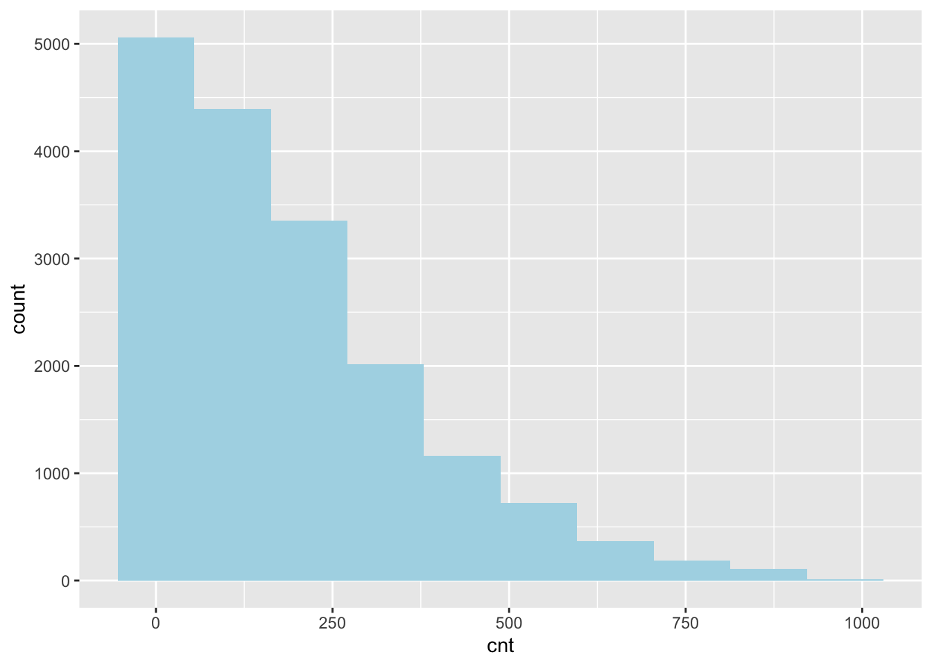

Question 2.5 {points: 3}

Since the number of bike rentals is strongly influenced by weather conditions, please create a scatterplot using ggplot to visualize the relationship between cnt (count of rentals) as a function of atemp (normalized feeling temperature in Celsius) on the x-axis and windspeed(normalized wind speed) on the y-axis. Use color to represent cnt values. add scale_colour_gradientn(colours = rev(hcl.colors(12))) as the last layer for your plot to specify a scale color from yellow to dark blue with 12 levels.

Comment on the relationship between the number of bike rental and temperature.

my_df |>
 ggplot()+
  geom_point(aes(x=atemp,y=windspeed,col=cnt)) +scale_colour_gradientn(colours = rev(hcl.colors(12)))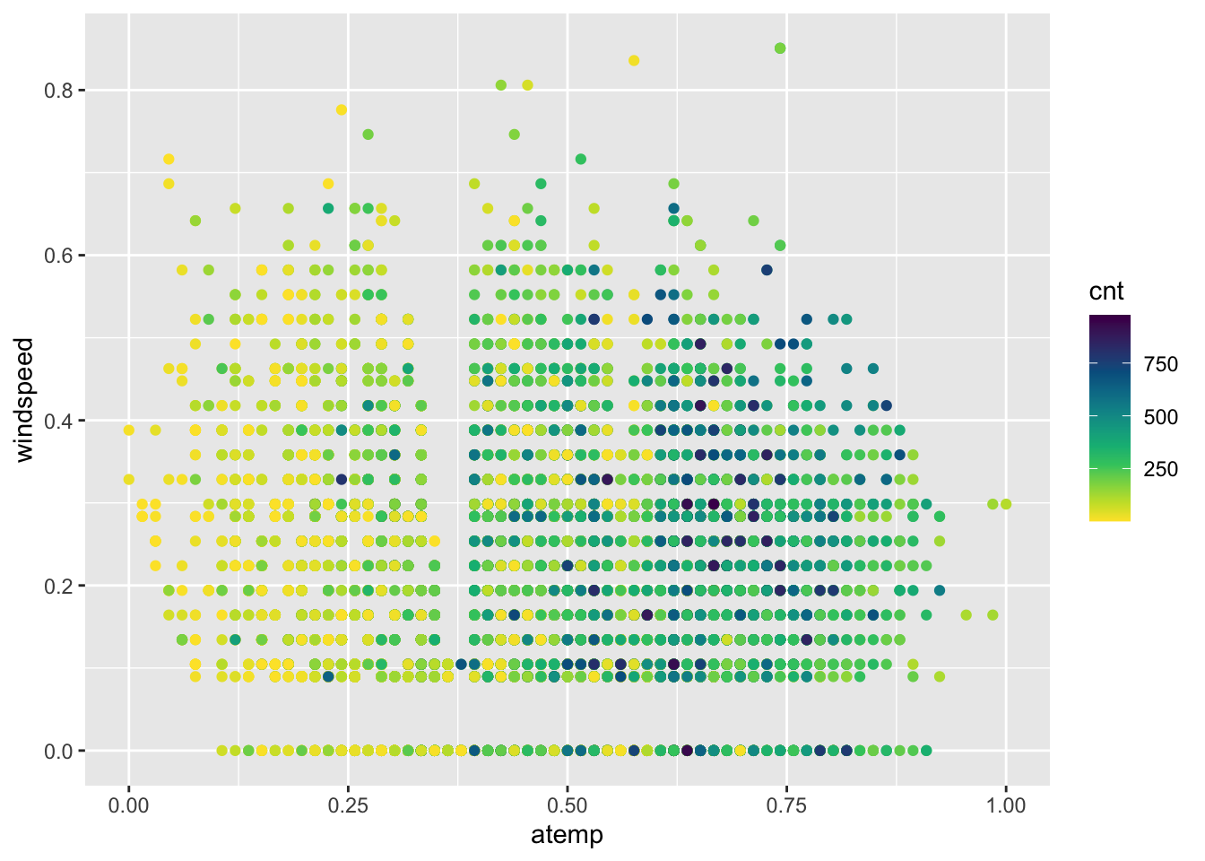

# the number of bike rentals increases with temperature.

Question 2.6 {points: 3}

Using tidymodels,split the my_df into training and testing set. Allocate 20% of the data to testing set. Make sure you set the proper arguments. Use set.seed(124)

set.seed(124)
bike_split <- initial_split(my_df, prop = 0.80, strata = cnt)
bike_training<- training(bike_split)
bike_testing<- testing(bike_split)

Question 2.7 {points: 2}

Create a recipe to formulate your model and preprocess your predictor variables.

bike_recipe<- recipe(cnt ~. , data = my_df) |>
  step_scale(all_predictors()) |>
  step_center(all_predictors())

Question 2.7 {points: 2}

Create a KNN regression model specification by using 3 nearest neighbors. call it knn_3.

knn_3 <- nearest_neighbor(weight_func = "rectangular", 
                                  neighbors = 3) |>
  set_engine("kknn") |>
  set_mode("regression")

Question 2.8 {points: 2}

Fit your KNN regression by creating a workflow by adding the recipe and model specification.

bike_fit_3<- workflow() |>
          add_recipe(bike_recipe) |>
          add_model(knn_3) |>
         fit(data = bike_training)

Question 2.9 {points: 3}

Now use the fitted model to make prediction on test data. Create a prediction dataframe (pred_3) by only including the actual count of bike rental and the predicted values.

pred_3 <- bike_fit_3 |>
           predict(bike_testing) |>
           bind_cols(bike_testing) |>
           select(cnt, .pred)
pred_3

# A tibble: 3,478 × 2
     cnt  .pred
   <dbl>  <dbl>
 1    40  12   
 2    56  46   
 3   110  28.3 
 4    67 331.  
 5     6   5.67
 6    20  44.3 
 7    70 205.  
 8    93 333.  
 9    22 104   
10     8  58   
# ℹ 3,468 more rows

Question 2.10 {points: 2}

Using base R function, calculate the Root Mean Squared Error for this prediction. Do you think your model performed well?

RMSE <- sqrt(mean((pred_3$cnt -pred_3$.pred)^2))
RMSE

[1] 176.4141

# this is a quite large error, it means our model did not perform best.

Question 2.11 {points: 10}

Now use 5-fold cross validation to find the best k. Create a tibble including the range of \(k\)s that contains the values 1, 3, 10, 25, 50,100, 200 and 500. Follow the steps outlines in the class and this tutorial.Ensure that you update your model specification and workflow as needed. Set the seed to 3456 for reproducibility.

Use collect_matrics to report the RMSE for each value of k. Which one would you choose?

set.seed(3456) 

k_vals <- tibble(neighbors = c(1,3, 10,25,100,200, 500)) #1 points
bike_cv_spec <- nearest_neighbor(weight_func = "rectangular", 
                                  neighbors = tune()) |>
  set_engine("kknn") |>
  set_mode("regression") # 2pints

bike_vfold <- vfold_cv(bike_training, v = 5, strata = cnt) # 1 point

bike_cv_wf <- workflow() |>
  add_recipe(bike_recipe) |>
  add_model(bike_cv_spec) # 1 points

bike_cv_results <- bike_cv_wf |>
  tune_grid(resamples = bike_vfold, grid = k_vals) |>
  collect_metrics() |>
  filter(.metric == "rmse") #4 points

bike_cv_results

# A tibble: 7 × 7
  neighbors .metric .estimator  mean     n std_err .config             
      <dbl> <chr>   <chr>      <dbl> <int>   <dbl> <chr>               
1         1 rmse    standard    204.     5   0.878 Preprocessor1_Model1
2         3 rmse    standard    174.     5   1.22  Preprocessor1_Model2
3        10 rmse    standard    159.     5   1.10  Preprocessor1_Model3
4        25 rmse    standard    154.     5   0.907 Preprocessor1_Model4
5       100 rmse    standard    153.     5   0.608 Preprocessor1_Model5
6       200 rmse    standard    153.     5   0.585 Preprocessor1_Model6
7       500 rmse    standard    154.     5   0.552 Preprocessor1_Model7

# they should choose k = 100 as it has the lowest RMS ( ~ 152.9912) # 1points

Text formatting Narrative and word answers should be typeset using regular text (as opposed to using using comments (preceded by #) within an R chunk. The use of of markdown formatting to improve readability is encouraged. Simple examples include:

• headers (second-level headers are preceded by ##)
• italics (*italics* or _italics_),
• bold (**bold**),
• typewritter text (`typewritter`)

Labels all HTML documents should satisfy the following criteria:

• assignments should be named assignment<x>_<y>.html where <x> is replaced by the assignment number and ` is replaced by your student number
• Your full name, student number, assignment number, and course number should appear somewhere near the top of the rendered document
• Questions should be labeled either by the use of headers or numbered lists.

Important

Submissions in any other format (e.g. Rmd, word document) will incur a 20% penalty.