Review Session 3

DATA 101: Making Prediction with Data

Authors

Affiliation

Introduction

Please ensure that you attend the section of the class for which you are registered. Both classes are at capacity and will not be able to accommodate students outside of our enrollment.

Date: Wednesday, November 22 (Irene’s section) / Thursday, November 23 (Ladan’s section)

Format: On paper, closed-book, in-person (no calculators/laptops/phones permitted).
Allowable material: Writing utensil, one cheat sheet (a standard sheet of paper front/back)
Duration: 80 minutes
Structure: a mixture of multiple-choice and short/long answer
Coverage: Lectures 9, 10, 11 and Lab 5 and 6

N.B. Your cheat sheet may be printed or hand-written

The structure of the quiz will be similar to Quiz 1 and 2. While there will be some conceptual and theoretical questions, the majority of points are associated with building, tuning, and evaluating a KNN classification model using tidymodels. Partial code will be given along the way.

Classification with \(k\)-nearest neighbours (KNN)

Classification

Classification involves predicting the value of a categorical variable (AKA class or label) using one or more variables. For instance predict the species of iris based on the numeric measurement data:

iris

plot(iris[,-5], col = iris[,5])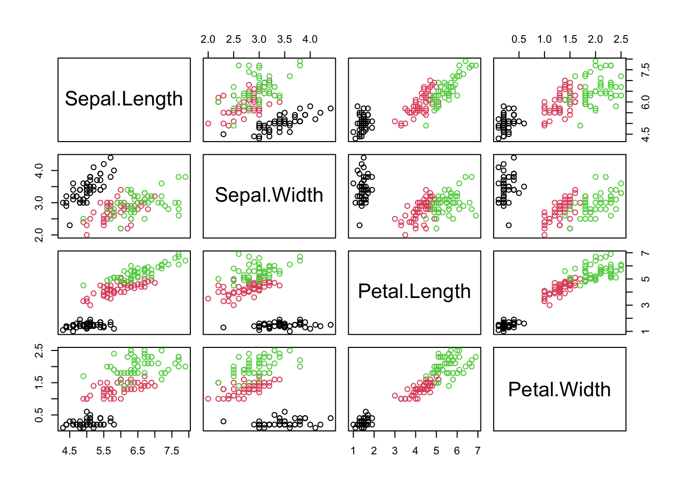

In this case our

output (or response) is species and
our predictors are: Sepal.Length, Sepal.Width, Petal.Length, Petal.Width (or some subset of these – we need not use all of them).

More generally classification relies on labeled data where the “label” is the class we are aiming to predict and the remainder (or some subset) of numeric or categorical variables, are used as predictors.

Training/Testing

The first step in fitting a model is to create training and test datasets from the original data.
The testing set provides an independent dataset to evaluate the performance of your model.
While we can do this using base R functions we will do this using tidymodels.
The most common split ratio is 70-30 or 80-20, where 70% or 80% of the data is used for training, and the remaining 30% or 20% is used for testing.
However, the choice of the split ratio may depend on the size of your dataset and the specific requirements of your analysis.

tidymodels

tidymodels is a collection of R packages for modeling and statistical analysis that follows the principles of tidy data and the tidyverse.
It provides a consistent workflow/format/notation across different types of machine learning algorithms
We can then easily modify preprocessing, algorithm choice, and hyperparameter tuning
Here is a typical pipeline linked to the variable packages within tidymodels

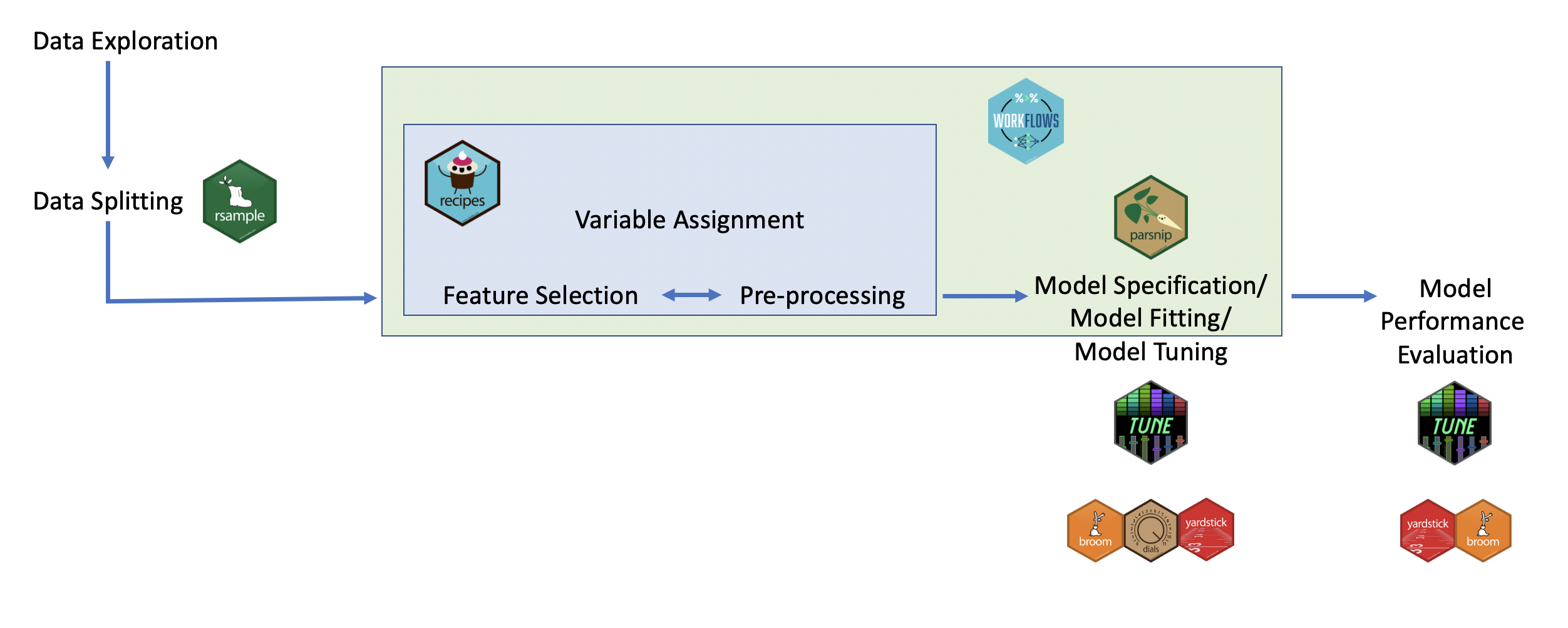
Source of image: Tidyverse skills for Data Science

rsamples - to split the data into training and testing sets (as well as cross validation sets - more on that later!)
recipes - to prepare the data with preprocessing (assign variables and preprocessing steps)
parsnip - to specify and fit the data to a model
yardstick and tune - to evaluate model performance
workflows - combining recipe and parsnip objects into a workflow (this makes it easier to keep track of what you have done and it makes it easier to modify specific steps)
tune and dials - model optimization (more on what hyperparameters are later too!)
broom - to make the output from fitting a model easier to read

N.B. we don’t and won’t pay too much to which package does what in the quiz/course

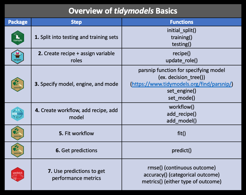
These are the major steps that we have covered:

Metrics

We can extract popular metrics for models using the metrics() function. In class we focus mostly on accuracy ; however, this is generally not the best metric.
Other metrics include:
- sensitivity (or recall): the proportion of all positive cases that were correctly classified
- specificity: the proportion of all negative cases that were correctly classified
These can all be calculated from a confusion matrix which has the form

	Actually Positive	Actually Negative
Predicted Positive	TP	FP
Predicted Negative	FN	TN

where

TP = true positives
TN = true negatives
FN = false negatives
FP = false positives

\[\begin{align*} \text{sensitivity} &= \frac{\text{TP}}{\text{TP + FN}} && \text{specificity} &= \frac{\text{TN}}{\text{TN + FP}} \end{align*}\]

A note about randomness …

Much of these pipelines rely on random splits of the data
In order to make our work reproducible it is very important that we set a seed (using set.seed())

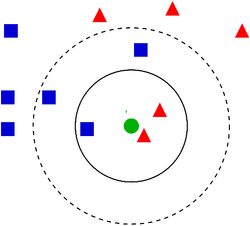
KNN

The goal of this classification algorithm is to produce non-overlapping regions where the same categorical outcome is predicted for all combinations of predictor values.

KNN Algorithm

Steps to the KNN classification algorithm

Choose the value of \(k\) (the number of “neighbors”)
Calculate the distances (usually Euclidean on scaled and centered training data)
Identify the \(k\) nearest neighbours (in training set)
Make predictions based on majority vote
Evaluate performance on the test set (e.g. using accuracy)

Pipeline

1. Data splitting

Using tidymodels we can split our data into training and testing using:

set.seed(2023)

set_split <- initial_split(dat, prop = p, strata = class)
train_data <- training(set_split)
test_data <- testing(set_split)

where p is the proportion of the data we want in our training set (and 1-p is the proportion that gets allocated to our test set).
if our classes are imbalanced (when the distribution of class labels is not roughly equal)
If our data is imbalanced we may want to use the following to ensure that the distribution in the ‘class’ variable is roughly the same in both the training and testing sets.

2. recipes (assign variable roles)

In tidymodels in R, we can specify a recipe using:

recipe(outcome~., data = training_data)

the first argument of recipe takes a formula of the form output_var ~ pred1 + pred2 + pred3..
The formula y~. is the shorthand way of saying that y is the outcome (target class) for our classification problem and the dot . is a placeholder for all other variables in the dataset. In other words, all remaining columns in our data frame will be used as a predictor.
```
# eg. on iris data:

recipe(Species~., data = training_data)

# same as

recipe(Species~ Sepal.Length + Sepal.Width +
        Petal.Length +  Petal.Width, data = training_data)
```
make sure the specification of the variables match how they appear in the data frame provided in the data argument

2. recipes (feature engineering)

Data pre-processing steps can be specified in our recipe using the appropriate step_*() function. Examples include:

centering and scaling numeric predictors (i.e. normalizing)
taking the log of numeric variables

For example to normalize all numeric predictors we could do:

my_recipe <- recipe(outcome~., data = training_data) %>% 
  step_scale(all_numeric_predictors()) %>% 
  step_center(all_numeric_predictors())

Note the other options for selectors: https://recipes.tidymodels.org/reference/has_role.html

(Optional) Pre-processing Step

If you want to see/store thenormalized data, we can examine it using prep() and bake(). This is not however necessary for the analysis and was only covered in lab

# train our recipe 
opt_prep <- my_recipe %>% 
  prep(training = training_data)

In our case, this would calculate the mean and standard deviation of the numeric columns. This will be used for centering and scaling data.

To apply the transformations formulas (as determined by the training set) to either the training and test datasets, we can use bake()

# Apply to training data
opt_prep %>% 
  bake(new_data = NULL)

# Apply to testing data
opt_prep %>% 
  bake(new_data = test_data)

Note the importnace of this step: our algorithms require the same data format as was used during model training to predict new values. In our case, we need to ensure that a new point in our test set gets transformed in the same way as was used in out training:

\[\begin{equation} \frac{x_1' - \text{mean}(X_1)}{\text{sd}(X_1)} \end{equation}\] where \(\text{mean}(X_1)\) and \(\text{sd}(X_1)\) was caluclated on the training set.

3. Specify model, engine, and mode

We need to define the following about our model:

The type of model (using specific functions in parsnip like rand_forest(), logistic_reg(), nearest_neighbors() etc.)
The engine, aka package, that we will use to implement the type of model selected
The mode of learning; either classification or regression

To find the settings for different models you can search: https://www.tidymodels.org/find/parsnip/

For this portion of the course and for the quiz we will be focused on \(k\) nearest neighbours classification. The algorithm goes as follows:

For KNN classification with 7 nearest neighbours for example we would use:

knn_spec <- nearest_neighbor(weight_func="rectangular", 
                             neighbors = 7) |>
  set_engine("kknn") |>
  set_mode("classification")

Recall that weight_func="rectangular" is something we use in this course to ensure each neighbour just counts as one vote towards the predicted class.

4. Create workflow

The workflows package allows us to keep track of both our preprocessing steps and our model specification.

my_workflow <-  workflow() |>
  add_recipe(my_recipe) |>
  add_model(knn_spec)

5. Fit workflow

We are now ready to fit the model:

my_fit <- my_workflow %>% 
  fit(data = training_data)

6. Get Predictions

Now that we have created our K-nearest neighbor classifier object, let’s predict the class labels for our test set. To make predictions we use the predict() function. Note that we can either obtain a predicted class or obtain the estimated probabilities for each category in the outcome variable

# Predict outcome categories
class_preds <- predict(my_fit, new_data = test_data,
                       type = 'class')

# Estimated probabilities for each outcome value
prob_preds <- predict(my_fit, new_data = test_data, 
                      type = 'prob')

It is helpful to store the results in a single data frame (to be used to obtain certain metrics)

my_results <- test_data %>% 
  select(outcome) %>%  # the true class label
  bind_cols(class_preds, prob_preds)

7. Performance metrics

We can now assess the model fit. For instance, to get a confusion matrix we could use:

cmat <- my_results |>
             conf_mat(truth = outcome, estimate = .pred_class)

While we can easily calculate things like accuracy, specificity, sensitivity, etc, from the confusion matrix we can also use some tidymodel functions from the yardstick package to do this for us:

# accuracy
my_results %>% 
  accuracy(outcome, estimate = .pred_class)

# sensitivity
my_results %>% 
  sens(outcome, estimate = .pred_class)

# specificity
my_results %>% 
  spec(outcome, estimate = .pred_class)

Alternatively, the popular metrics of accuracy can be extracted using:

my_results |>
  metrics(truth = outcome, estimate = .pred_class) |>
  filter(.metric == "accuracy")

Tuning

The vast majority of predictive models in statistics and machine learning have parameters that you have to pick.
These are called tuning parameters
In the case of KNN classification, the tuning parameter is \(k\).
Rather than arbitrarily selecting a value for \(k\), we can instead choose it using cross-validation

Cross-validation

This method involves essentially preforming the holdout method iteratively with the training data.

We can perform a cross-validation in R using the vfold_cv function. Again, because these are created at random, we need to use the base set.seed() function in order to obtain the same results each time.

set.seed(2023)
my_vfold <- vfold_cv(training_data, v = n_folds)

where n_folds is the number of desired folds. This is often 5 or 10 (we usually specify in the question how many folds we want).

Now perform the workflow analysis again, this time for a series of candidate values for \(k\). We will store that in a tibble:

# examples of grids for k:
k_vals <- tibble(neighbors = seq(from = 1, to = 10, by = 1))
k_vals <- tibble(neighbors = seq(from = 3, to = 100, by = 5))

Recall that in our previous model specification, we (arbitrarily) set \(k\) = 7. We need to update our workflow to allow for this grid of potential \(k\) values to be used:

knn_tune <- nearest_neighbor(weight_func = "rectangular", 
                             neighbors = tune()) |> # no longer 7
  set_engine("kknn") |>
  set_mode("classification")

updated_workflow <- workflow() |>
       add_recipe(my_recipe) |> # normalize predis/outcome the same
       add_model(knn_tune)

Now let’s refit the modelS:

updated_fit <- updated_workflow |>
       tune_grid(resamples = my_vfold, grid = k_vals)

Note how we use tune_grid Instead of using fit (or fit_resamples which we can use with cross-validation for a particular value of \(k\)).
We will use the tune_grid function to fit the model for each value in a range of parameter values (stored in k_vals.
The resamples argument takes the cross-validation my_vfold object we created earlier.
The grid argument specifies that the tuning should try \(k\) = k_vals[1], then \(k\) = k_vals[2], …
We can then collect the metrics estimated for each of the different values of \(k\) using the collect_metrics() function:

cv_results <- updated_fit %>% 
  collect_metrics()

It is often useful to extract the accuracies from this to visualize quickly where our “best” choice for \(k\) is.

accuracies <- cv_results %>% filter(.metric == "accuracy")

ggplot(accuracies, aes(x = neighbors, y = mean)) +
  geom_point() +
  geom_line() +  scale_x_continuous(breaks = unique(k_grid$neighbors)) +
  labs(y = "accuracy")

Generally speaking, the value(s) of \(k\) that obtain the highest accuracy is going to be the “best” choice(s) for the number of nearest neibours. Once we decide on that value we would return to step 3 and rerun the analysis with the neighbors argument set to best \(k\) as determined by cross-validation.

best_k = accuracies %>% 
  slice_max(order_by = mean) %>%
  pull(neighbors)

best_acc = accuracies %>% 
  slice_max(order_by = mean) %>%
  pull(mean)

Example

Let’s work through the example from your assignment…

library(tidymodels)

mobile_carrier_df <- 
  readRDS(url('https://gmubusinessanalytics.netlify.app/data/mobile_carrier_data.rds'))
str(mobile_carrier_df)

tibble [2,277 × 14] (S3: tbl_df/tbl/data.frame)
 $ canceled_plan                : Factor w/ 2 levels "yes","no": 1 2 1 2 2 1 2 1 2 2 ...
 $ us_state_region              : Factor w/ 9 levels "East North Central",..: 1 7 5 7 4 1 2 3 4 7 ...
 $ international_plan           : Factor w/ 2 levels "no","yes": 1 1 1 1 1 1 1 2 2 1 ...
 $ voice_mail_plan              : Factor w/ 2 levels "no","yes": 1 2 1 1 2 1 2 1 2 1 ...
 $ number_vmail_messages        : int [1:2277] 0 11 0 0 33 0 28 0 30 0 ...
 $ total_day_minutes            : num [1:2277] 202 253 113 139 228 ...
 $ total_day_calls              : int [1:2277] 105 129 108 107 85 106 117 106 114 101 ...
 $ total_eve_minutes            : num [1:2277] 195 284 169 257 249 ...
 $ total_eve_calls              : int [1:2277] 131 88 107 113 114 109 102 99 106 95 ...
 $ total_night_minutes          : num [1:2277] 190.1 262.8 156.6 234.9 93.5 ...
 $ total_night_calls            : int [1:2277] 88 99 61 74 89 93 80 89 105 123 ...
 $ total_intl_minutes           : num [1:2277] 9 12.3 9.2 10 10.2 8.7 8.7 8.5 12.9 9.3 ...
 $ total_intl_calls             : int [1:2277] 2 1 5 3 7 3 3 3 3 4 ...
 $ number_customer_service_calls: int [1:2277] 3 1 2 0 0 0 0 6 2 2 ...

In this dataset, each row corresponds to a customer and indicates whether they terminated their service. The output (aka target aka response) variable is canceled_plan. As we can see, it is properly coded as a factor with two levels: "yes" or "no".

Notice that the data is NOT balanced (aka imbalance/unbalanced):

bar_gg <- ggplot(mobile_carrier_df)+
          geom_bar(aes(x=canceled_plan), fill = 'lightblue')+
          labs(x = "Customer canceled their plan", y = "Number of cases")+ theme_classic()
bar_gg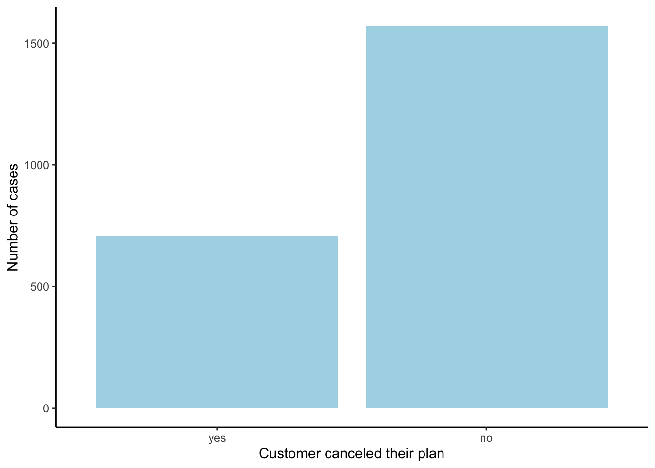

1. Data splitting

Allocate 80% of data points to the training set. Ensure that the split maintains the category proportions within each subset.

mobile_split <- _______________(mobile_carrier_df, prop = 0.8,
                              
                                strata = _____________________)

Code

mobile_split <- initial_split(mobile_carrier_df, prop = 0.8,
                              strata = canceled_plan)

Create a training and testing set:

# Create the test data
mobile_test <- ___ %>% 
  ___

Code

mobile_test <- mobile_split %>% 
  testing()

# Create the test data
mobile_training <- ___ %>% 
  ___

Code

mobile_training <- mobile_split %>% 
  training()

# or (without the pipes:)

mobile_training <- training(mobile_split)

2. Recipes

Create a recipe by using only numeric variables for the predictors and canceled_plan as the response variable.

mobile_recipe <- recipe(_________________________________ , 
                        
                        data = ___________________________) |>
  
  __________________________________

Code

my_formula <- formula(canceled_plan ~ number_vmail_messages+total_day_minutes+total_day_calls+total_eve_minutes+total_eve_calls+total_night_minutes+total_night_calls+total_intl_minutes+total_intl_calls+number_customer_service_calls)

mobile_recipe <- recipe(my_formula , data = mobile_training) |>
  step_scale(all_numeric_predictors()) |>
  step_center(all_numeric_predictors())

which is the same as:

Code

recipe(canceled_plan ~ number_vmail_messages +
                          total_day_minutes + total_day_calls + 
                          total_eve_minutes + total_eve_calls + 
                          total_night_minutes + total_night_calls + 
                          total_intl_minutes + total_intl_calls + 
                          number_customer_service_calls, 
                    data = mobile_training) |>
  step_scale(all_numeric_predictors()) |>
  step_center(all_numeric_predictors())

Which is the same as:

Code

recipe(canceled_plan ~ number_vmail_messages +
                          total_day_minutes + total_day_calls + 
                          total_eve_minutes + total_eve_calls + 
                          total_night_minutes + total_night_calls + 
                          total_intl_minutes + total_intl_calls + 
                          number_customer_service_calls, 
                    data = mobile_training) |>
  step_scale(all_predictors(), -all_outcomes()) |>
  step_center(all_predictors(), -all_outcomes())

3. Model specification

Since we don’t know what an optimal \(k\) will be, let’s first specify a grid of candidate models.

# vector of possible k values 
k_vals <- tibble(neighbors =c(5, 10, 15, 25, 45, 60, 80, 100))

Since we know we’ll need to use cross-validation to pick the “best” \(k\), let’s created our 6-fold cross-validation split of our training data.

# folds used in cross-validation 
set.seed(271)
mobile_folds <- _____________(________________________
                                   , v = __________)

Code

# folds used in cross-validation 
set.seed(271)
mobile_folds <- vfold_cv(mobile_training, v = 6)

Recall usage of this function

vfold_cv(data, v = 10,  strata = NULL)

if we don’t specify the number of partitions we desire, 10-fold cross-validation will be done by default
like with initial_split we have a strata argument.

Although we didn’t ask you to do this on the assignment, when we have umbalanced data it is probably a good idea to set this to the outcome variable to ensure that each fold has a similar distribution of the specified strata variable as the overall dataset.

mobile_folds <- vfold_cv(mobile_training, v = 6, 
                         
                         strata = __________________________)

Code

# folds used in cross-validation stratified by
set.seed(271)
mobile_folds <- vfold_cv(mobile_training, v = 6, strata = canceled_plan)

Now we want to specify our model. If you forget any model types, engines, and arguments go here: https://www.tidymodels.org/find/parsnip/

knn_spec <- ______________________(                               # type (model function name)
                           _______________________,               # optional arguments
                           ________________________) |>           # required arguments

               set_engine( ___________) |>                        # engine

               set_mode(________________)                         # mode

Code

knn_spec <- nearest_neighbor(neighbors = tune()) |>                  # type
             set_engine('kknn') |>                                   # engine
             set_mode('classification')                              # mode

When looking at the documentation for the nearest_neighbor type, we can that we have an optional argument weight_func that

A single character for the type of kernel function used to weight distances between samples. Valid choices are: "rectangular", "triangular", "epanechnikov", "biweight", "triweight", "cos", "inv", "gaussian", "rank", or "optimal".

As discussed in class, we want to use: weight_func = "rectangular" which assigns equal weight to all neighbors within the specified k.

knn_spec <- nearest_neighbor(weight_func = "rectangular",
                             neighbors = tune()) |>                  # type
             set_engine('kknn') |>                                   # engine
             set_mode('classification')                              # mode

knn_spec

K-Nearest Neighbor Model Specification (classification)

Main Arguments:
  neighbors = tune()
  weight_func = rectangular

Computational engine: kknn

4. Create workflow

The workflows package allows us to keep track of both our preprocessing steps and our model specification

knn_wf <- workflow() |>                           # start with worflow function
          add_<_________>(_____________) |>       # add the model
          add_<_________>(______________)         # add the recipe

Code

knn_wf <- workflow() |>
          add_model(knn_spec) |>
          add_recipe(mobile_recipe)

Tune the model

Now we need to perform hyperparameter tuning in order to find out the best choice for \(k\). To do this we use the tune_grid function. It’s typically applied within a workflow to search over a grid of hyperparameter values and find the combination that results in the best model performance based on a specified metric.

cv_fit <- __________________ |>                     # apply to our saved workflow
  tune_grid(resamples = __________________,         # the cross-validated folds
            grid = _______________________)         # vector of candidate k values

Code

set.seed(314)
cv_fit <- knn_wf |>                                # apply to our saved workflow
  tune_grid(resamples = mobile_folds,              # the cross-validated folds
            grid = k_vals)                         # vector of candidate k values

The tune_grid() function fits models for each possible value of hyperparameter values as specified in grid. It uses resampling (e.g., cross-validation) to assess the model performance. To exract the estimated accuracies of each of these models we can use the collect_metrics() function

collect_metrics(cv_fit)

As mentioned in class, these provides two metrics: the accuracy and roc_auc, but we only care about accuracy in this course. So lets extract that information and store it to a new data frame.

cv_results <- collect_metrics(cv_fit) %>% 
  filter(.metric == 'accuracy') # keep only the rows that provide ests of accuracy

cv_results

It is useful to plot this data

ggplot(_________________, aes(x = ___________, y = ________________)) +
      geom_<_____________________>() +
      geom_<___________________>() +  
      # to coincide with our choices for k
      scale_x_continuous(breaks = unique(k_vals$neighbors)) +
      labs(___________________________)

Code

ggplot(cv_results, aes(x = neighbors, y = mean)) +
      geom_point() +
      geom_line() +  scale_x_continuous(breaks = unique(k_vals$neighbors)) +
      labs(y = "accuracy")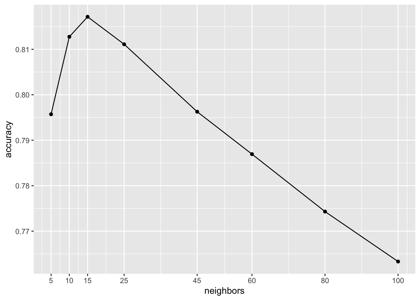

We can read the best \(k\) from the plot or code it for a more automated approach

cv_results %>% arrange(mean)

we can make use of the slice_* function which lets you index rows certain criteria

cv_results %>% slice_max(order_by = mean)

best_k = cv_results %>% slice_max(order_by = mean) %>%
      pull(neighbors) # pull() is like using $
best_acc = cv_results %>% slice_max(order_by = mean) %>%
      pull(mean)

c(best_k, best_acc)

[1] 15.0000000  0.8171494

The best \(k\) is 15 which obtains an estimated accuracy of 0.8171494

5. (re)Fit the model

Now we need to refit the model with that specification of \(k\). That is our tuning parameter can now be set to the “best” choice as determined by cross-validation.

We need to update our model specification

bestknn_spec <- nearest_neighbor(neighbors = best_k) |>
      set_engine("kknn") |>
      set_mode("classification")

Now we can refit the model using:

mobile_fit <- workflow() |>
  add_recipe(mobile_recipe) |> # reused from before
  add_model(bestknn_spec) |>   # updated to a certain k
  fit(data = mobile_training)  # remember to still use the training data

6. Predict

FINALLY! we can use our fitted model to predict “new” observations in the form of our preserved test set. To do this we use our predict() function

# Predict outcome categories
(class_preds <- predict(mobile_fit, new_data = mobile_test,
                       type = 'class'))

# Estimated probabilities for each outcome value
(prob_preds <- predict(mobile_fit, new_data = mobile_test, 
                      type = 'prob'))

The default is to give the class prediction (in this case “yes” or “no”)

predict(mobile_fit, mobile_test)

To help in the next section, lets store the predicted class in the same data frame as the true class:

test_prediction <- predict(mobile_fit, mobile_test) |>
  bind_cols(mobile_test) 

test_prediction

7. Assess

To assess our model we can look at the confusion matrix:

confusion_mat <- test_prediction |> conf_mat(truth = canceled_plan, estimate = .pred_class)

confusion_mat

          Truth
Prediction yes  no
       yes  75  17
       no   67 297

We can calucate

\[\begin{align*} \text{sensitivity} &= \frac{\text{TP}}{\text{TP + FN}} && \text{specificity} &= \frac{\text{TN}}{\text{TN + FP}} \end{align*}\]

While we can easily calculate things like accuracy, specificity, sensitivity, etc, from the confusion matrix we can also use some tidymodel functions from the yardstick package to do this for us:

# accuracy
test_prediction %>% 
  accuracy(canceled_plan, estimate = .pred_class)

# sensitivity
test_prediction %>% 
  sens(canceled_plan, estimate = .pred_class)

# specificity
test_prediction %>% 
  spec(canceled_plan, estimate = .pred_class)