Data 311: Machine Learning

Lecture 13: Classification and Regression Trees

Dr. Irene Vrbik

University of British Columbia Okanagan

Introduction

• We have some of the basics for building/assessing models

• Much of the remainder of the course we will be introducing some new models; today’s topic is tree-based methods.

• Tree-based methods are simple and useful for interpretation; however, they are typically are not competitive with the some of the alternative approaches we’ll be discussing

• each lecture from here on out will be a self-contained topic
• simple and useful for interpretation.
• not competitive
• combining a large number of trees can often result in dramatic improvements in prediction accuracy, at the expense of some loss in interpretation.

Next lecture (bagging, random forests and boosting) involves using multiple trees and combining them to yield a more competitive result.

CART

• Classification and Regression Trees (AKA CART or decision trees) involve partitioning (AKA stratifying or segmenting) the predictor/feature space by simple binary splitting rules.

• Since the set of splitting rules used to segment the predictor space can be summarized in a tree, these types of approaches are known as decision tree methods.

• We make a prediction for an obs. using the mean/mode response value for that “region” to which it belongs.

• Started in mid-80s CART first software package
• tree-based methods involve stratifying or segmenting the predictor space into a number of simple regions.
• think flow chart (only binary discussions)
  • twenty questions analogy
  • find the answer in the fewest questions
• what are the best questions to ask –> what are the best splits to use

Motivating Classification Example

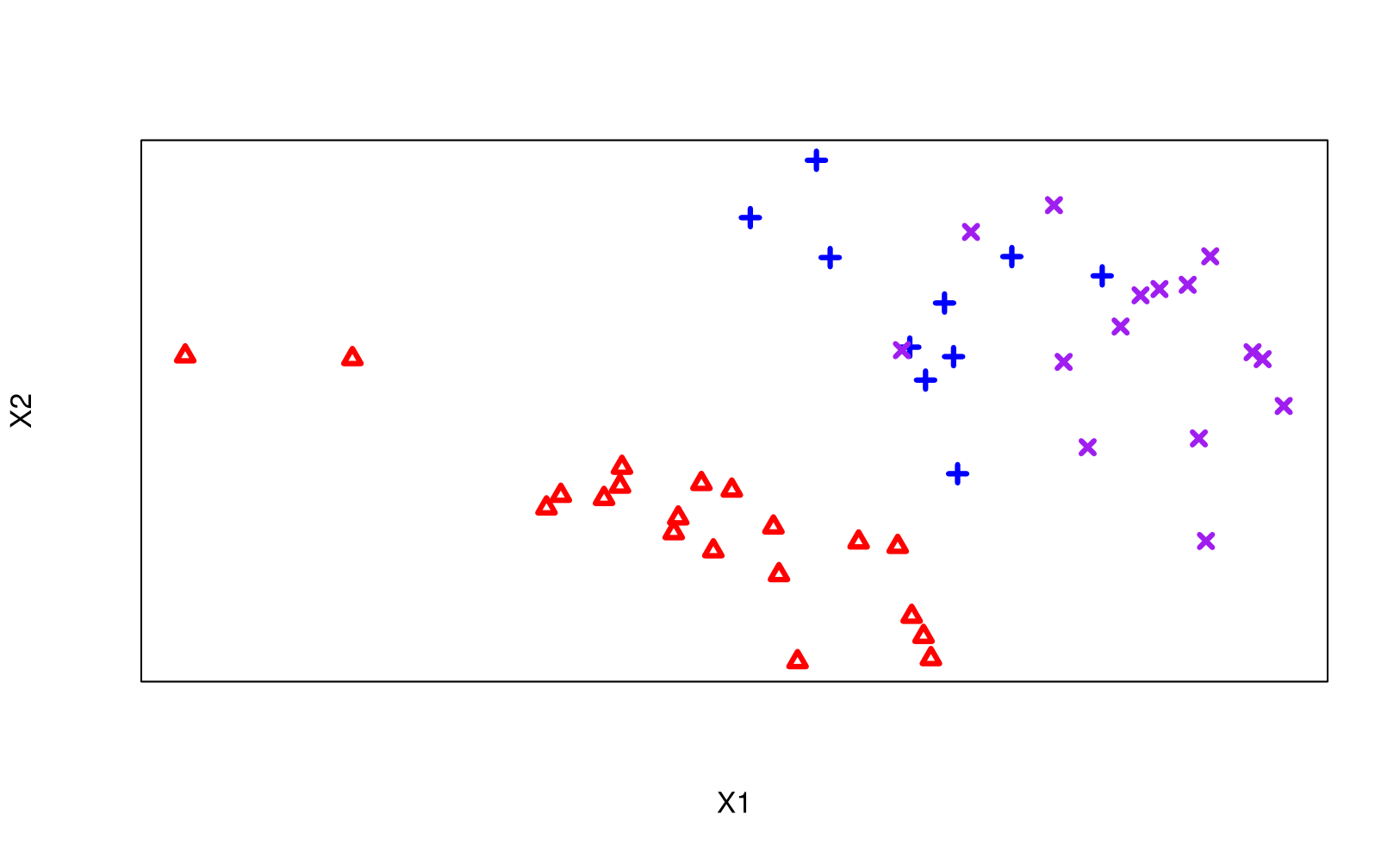
Task: partition the feature space into subsets, with each subset/region corresponding to a specific class.

True classes are colour/shape-coded

Rules: Regions can only be split horizontal or vertically.

• Decision trees can be applied to both regression and classification problems.
• We will look at two motivating examples one in classification and one in regression
• Be efficient: goal of maximizing the homogeneity of the child nodes (regions) in terms of the target variable (class).
• restrict to vertical and horizontal cuts (binary decisions on a feature variable)

First Rule on X1

As a first go, let this line represent a decision

• restrict to vertical and horizontal cuts (binary decisions on a single variable)
• if a point lies on the left of this line, we’ll predict a red triangle, but i have more work to do on the right
• Be efficient: goal of maximizing the homogeneity of the child nodes (regions) in terms of the target variable (class).

Rule 1:

Let’s summarize this as a flow chart:

• left = yes right = no (intuitive!)
• Still got more work to do if x>a

Second Rule on X1

the left-most region is said to be pure (i.e. only containing observations from the red triangle group; see Gini Index)

• create an additional split at b
• to the right of b, i’ll predict purple x (one blue + but maybe ok)
• less than b, more work

Rule 2

Third Rule on X2

• if less than c –> red triangle
• if grater than c blue +
• predict points falling in some boxed region
• each region corresponds to a terminal node in our tree

Rule 3

The prediction at a terminal node is the majority class for that corresponding region in the feature space.

• these terminal node predictions are simply just the majority class in that region (similar to knn-classification)

Tree Notation

To aid with notation, try to visualize this flow chart as an upside-down binary tree with a set of connecting nodes:

• The root node represents the entire population or sample and sits base of the tree.

• A nodes that splits is called an internal node or decision node and is said to be the parent to its left/right child.

• A node that does not split is a terminal node, or leaf.

• A sub-section of an entire tree is called branch.

• terminal nodes correspond to \(R_j\)s

Notation (on tree)

• Terminal node = leaves (red, purple, blue)
• upside-down tree
• yellow node AKA decision notes/internal nodes
• terminal nodes correspond to \(R_j\)s

Upside-down tree

Image adjusted from: medium.com

• 7 is parent to node 6 and 8

• 7 is a child to node 9

• There are multiple branches (i.e. sub-trees) we can highlight

When do we stop?

• Back to our motivating Classification example…

• We could make more binary rules such that nothing gets misclassified …

• … or could we be done with our Third Rule on X2?

8 Regions

• defines eight regions
• Each region is ‘pure’ in that it contains only observations from a single class.

Question: at this point, you should be concerned with …

• A: overfitting

Question: when do we stop?

• common rules to come.

Motivating Example: Comments

• So, it appears there are some things we may need to consider going forward in the classification realm.

• Before diving further into specifics, let’s motivate trees for regression through an example.

• Our regression tree will be built by spliting \(X\) into partitions (or branches), and iterartively splitting partitions into smaller partitions as we moves up each branch.

• y is continuous now
• For simplicity we consider only a single predictor variable X.

Motivating Regression Example

for simplicity one predictor

Split 1

• flow chart will be similar except terminal nodes will be values for Y rather than classes
• to the left of a pretty homogenous
• right of a we have some work to do
• split the right hand side into regions of homogeneity

Split 2

• b splits into high variance and low variance
• we probably won’t be able to predict in the area to the left of b very well

Split 3

• we continue (eye-balling) splits into similarly behaved regions

Split 4

• let’s stop by selection this last area of high variability
• Once we think it’s reasonable to stop, now what?

Predictions?

• Now that we have (five) regions of relative homogeneity in \(Y\)…what would the simplest plan be?

• Easy solution is to average the observations in the region to provide the predicted value for every observation that falls into the region \(R_j\).

• More generally, in order to make a prediction for a given observation, we typically use the mean or the mode response value for the training observations in the region to which it belongs.

\(Y\) Predictions

• so if i have a x < i predict…
• we can again draw a flow chart (but i wont) with termal notes = values
• each rectange is a region that corresponds to a terminal node

Baseball Example:

Figure 1: Hitters dataset from Major League Baseball player data from 1986-87. y-axis: number of years playing in the major leagues. x-axis: number of hits in the previous year. Colour: salary (low salary is blue/green, and the high salary is red/yellow)

• Years is the most important factor in determining Salary, and players with less experience earn lower salaries than more experienced players.
• Given that a player is less experienced, the number of Hits that he made in the previous years seems to play little role in his Salary.
• But among players who have been in the major leagues for five or more years, the number of Hits made in the previous year does affect Salary, and players who made more Hits last year tend to have higher salaries.
• Surely an over-simplification, but compared to a regression model, it is easy to display, interpret, and explain.

Steps

• Divide the predictor space (\(X_1\), \(X_2\), , \(X_p\)) into \(J\) non-overlapping regions¹ \(R_1, R_2, \ldots, R_J\).

• For every observation that falls into the region \(R_j\) , we make the same prediction:

  • Regression: Predict the mean response for the observations that fall into each region \(R_j\).

  • Classification: Predict the categorical response as the most commonly occurring (i.e. mode) in each region \(R_j\).

• gardening background is an asset
• In theory, the regions could have any shape but we stick to boxes because they are simple and easy to interpret

1. In theory, the regions could have any shape, but we use high-dimensional rectangles, or boxes, for simplicity and for ease of interpretation.

Growing a Tree

Details on

• how to define a good split
• when to know when to stop

Goal

To “grow” our tree, i.e. to determine our splitting rules, we use a top-down (greedy) approach called recursive binary splitting.

1. It starts with all observations in a single region then splits the predictor space into two.

2. Then, one of those two regions are split in two (now we have three regions).

3. Then one of those three regions are split it two, …

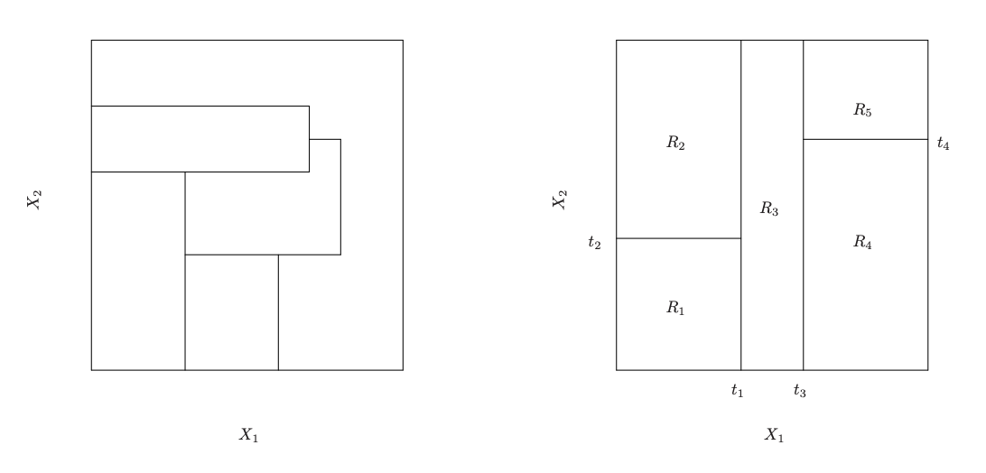
Im/Possible Regions

Left: A partition of two-dimensional feature space that could not result from recursive binary splitting. Right: The output of recursive binary splitting on a two-dimensional example.

Resulting Tree

The tree (left) corresponding to the feature space partition (right).

Growing a Tree (Regression)

• How do we pick a “good” split of the predictor space?

• For regression the goal is to find the regions \(R_1, \dots R_J\) which minimize the RSS given by: \[RSS = \sum_{j=1}^J \sum_{i \in R_j} (y_i-\hat y_{R_j})^2\] where \(\hat y_{R_j}\) is the mean response for the training observations within the \(j\)th region; see Recursive Binary Splitting.

• \(\hat y_{R_j}\) was the average of the obs in the \(R_j\) (horizontal red lines in previous plot)
• where \(J\) is the number of non-overlapping hyper-rectangles that partition the predictor space.

Determining the first split

• However, we cannot consider all possible hyper-rectangles in our data-set to find the optimal tree; jump to example

• Instead, we can start seek predictor \(X_j\) and cutpoint \(s\) such that the following is minimized with the resulting regions:

\[\begin{equation} \sum_{i: x_i \in R_1(j, s)} (y_i - \hat y_{R_1})^2 + \sum_{i: x_i \in R_2(j, s)} (y_i - \hat y_{R_2})^2 \end{equation}\]

\[\begin{align} R_1(j, s) &= \{X\mid Xj < s\} & R_2(j, s) &= \{X\mid Xj ≥ s\} \end{align}\]

• Choose the set of boxes s.t. the total variations of ovesrvations around their mean in a box is as small as possible
• Makes sense since make the boxes as homogeneous as possible
• computationally impossible as dimensionality increases
• build this tree recursively
• A similar argument can be made for classification with the Gini index for example.

where \(\hat y_{R_i} = \text{mean response in } R_i(j,s)\)

Determining the next split

• Then, via the same process, we either subdivide region \(R_1\) or \(R_2\) (whichever one leads to the greatest reduction in RSS), so that we have 3 regions: \(R_1\), \(R_2\), \(R_3\)

• Then we split one of these three regions further, …

The process continues until a stopping criterion is reached.

jump to example

General: consider all predictors \(X_1, . . . , X_p\), and all possible values of the cutpoint \(s\) for each of the predictors, and then choose the predictor and cutpoint such that the resulting tree has the lowest RSS.

• this can be done quite quickly, especially when the number of features p is not too large.
• as we did in the motivating example, we only build one rule at a time, or one cut
• this does not guarantee we find the best possible partition

Recursive Binary Splitting

• This process of recursive binary splitting is known as a greedy approach

• It’s greedy since it does not anticipate splits that will lead to a better tree in some future step, it only does the best decision at that particular step.

• Consequently, this greedy approach does not ensure we find the best tree (in terms of minimum RSS) but it is computationally feasible

this does not ensure we find the best tree (but hopefully a good one) - again each case we’re doing the best we at this particular moment

Stopping Criterion

We may continuing splitting until, for example:

1. each region contains fewer than, say, 5 observations
2. the change in the RSS is less than some \(\epsilon\)

Strategy 2 tends to produce smaller trees, but is too short-sighted. So typically we grow a larger tree than needed which we can potentially prune back.

• option 2 may lead us to stop prematurely (a so-so split could potentially be followed by a very good split)
• so we typically like to make a big (“bushy”) tree and then prune it (but it back)
• if we force a minimum of 3 obs on regression example, we get lots of small boxes
• making a big a tree as possible will be too much since that will definately overfit

Note that the RSS will always go down as we sub-divide.

Growing a Tree (Classification)

• For classification minimizing the misclassification rate is not usually done at the growth stage as it is too “jumpy”.

• Instead, usually the Gini index, deviance, or cross-entropy is used to evaluate the quality of a particular split¹

• Numerically these are very similar and most of the time, it won’t make a large difference which you use.

N.B. when pruning the tree (more on this in a second) we will typically use classification error rate.

• turns out the misclassifcation rate is very jumpy and noisy so it doesn’t lead to a very smooth tree growing process
• misclassification rate does not lead to a strictly concave purity function guaranteeing the uniqueness of the optimum at each split. This property, while not absolutely essential from a statistical point of view, is useful from a computational point of view by avoiding ties for the best split selection. [Random Forests with R, pg 12]
• we’ll pick the split that makes the metric go down the most
• the deviance is negative two times the maximized log-likelihood (defined on page 353)
• numerically they are all pretty close

1. These approaches are more sensitive to node purity than is the classification error rate.

Gini Index

The Gini index defined below is a measure of node inpurity¹

\[G = \sum_{k=1}^K \hat p_{mk} (1-\hat p_{mk})\] where \(K\) is the number of response classes, and \(\hat p_{mk}\) is the proportion of training observations in the \(m\)th region that are from the \(k\)th class

• if node \(m\) contains observations predominantly from a single class.

• The gini index is defined for each node [pg 12]

• [blog] good visuals but i think the math is wrong! (recreate for lab properly)

1. G is 0 if all \(\hat p_{mk}\) are zero or one, i.e. if all nodes are pure. A Gini index of 0.5 denotes equally distributed elements into \(K\) classes.

Cross Entropy

An alternative to the Gini index is the cross-entropy, given by \[\begin{equation} D = - \sum_{k=1}^K \hat p_{mk} \log \hat p_{mk} \end{equation}\]

or the residual mean deviance (or simply deviance) given by: \[\begin{equation} -2 \sum_m \sum_k n_{mk} \log \hat p_{mk} \end{equation}\]

where \(n_{mk}\) is the number of observations in the \(m\)th terminal node that belong to the \(k\)th class.

• The deviance generalizes the Residual Sum of Squares (RSS) of the linear model
• deviance is closely related to entropy and practically spearing they are all numerically very simialr and don’t make much of a difference
• deviance is negative 2 times the log likelihood and end up in the case of least squares the deviance and the residual sum of squares are equivalent source
• but for other model types the deviance is really just a generalization or residual sum of squares but here we’re

Pruning

Problem

• Building a tree through the description just given will tend to overfit¹ to the training data and lead to poor test set performance.

• A common strategy is to grow a large tree, \(T_0\), and then prune it back to obtain a subtree.

• Intuitively, our goal is to select a subtree that leads to the lowest test error rate.

A good StatQuest video on the subject.

• prune - gets a subtree
• is your tree too “bushy”?
• too small regions,
• splits leading to the same prediction,
• Prune it down

1. In other words, we will tend to build too large/complex a tree

Cross-validation

• Given a subtree, we can estimate its test error using cross-validation or the validation set approach.

• However, estimating the cross-validation error for every possible subtree would be too cumbersome, since there is an extremely large number of possible subtrees.

• Instead, of considering every possible subtree, we select a small set of subtrees for consideration using cost complexity pruning ¹

test error measured by MSE for example for regression

1. also is known as weakest link pruning

Cost Complexity Pruning

We consider a sequence of trees indexed by a non-negative tuning parameter \(\alpha\). For every value of \(\alpha\) there corresponds a subtree, \(T \in T_0\), such that the following is minimized: \[\begin{equation} \sum_{m=1}^{|T|} \sum_{i:x_i \in R_m} (y_i - \hat y_{R_m})^2 + \alpha |T| \end{equation}\]

• Here \(|T|\) is the number of terminal nodes in the tree,
• \(R_m\) is the region corresponding to the \(m\)th terminal node
  
• \(\hat y_{R_m}\) is the mean of the training observations in \(R_m\).

• minimize the RSS but penalize this criterion according to the size of the tree
• bigger trees will have a smaller RSS but larger penalization
• \(\alpha\) inflates the RSS according to the size of the tree
• we choose an optimal value of \(\hat \alpha\) using cross-validation
• We then return to the full data set and obtain the subtree corresponding to \(\hat \alpha\)

Tuning Parameter

• When \(\alpha = 0\), then the subtree \(T\) will simply equal \(T_0\)

• However, as \(\alpha\) increases, there is a price to pay for having a tree with many terminal nodes, and so the penalized RSS will tend to be minimized for a smaller subtree.

• In that way, \(\alpha\) controls the trade-off between the subtree’s complexity and its fit to the training data.

• It turns out that as we increase \(\alpha\) from zero, branches get pruned from the tree in a nested and predictable fashion.

1. because then (8.4) just measures the training error.

• whats the optimal \(\alpha\)? ans: use cv to tell you
• when \(\alpha=0\) there is no penalty to tree size, so we choose the biggest one
• as \(\alpha\) increases we put more and more penalty on tree size until there are one node (no splits)
• so tree size is inversely proportional to \(\alpha\)

Picking \(\alpha\) using CV

• Using \(k\)-fold cross validation, we both build trees, and prune them back for possible values of \(\alpha\)

• Each tree and subtree built in this fashion will produce an estimate of the MSE.

• Pick the \(\alpha\) that minimizes the predicted MSE using the above cross-validation.

• Then prune the original tree (built on the full data) with the chosen \(\alpha\).

https://www.youtube.com/watch?v=D0efHEJsfHo&ab_channel=StatQuestwithJoshStarmer 1. Fit full tree on all of the data - 0 = full tree. - Now, increase \(\alpha\) until pruning leaves will give us a lower tree score (penalized RSS) - increase \(\alpha\) again until pruning leaves gives us a lower tree score Different values of \(\alpha\) give us a sequence of trees from full sized to just a leaf (stub) 2. Divide data into k-folds. For each k,…. On training: - Use the \(\alpha\) values from previous step to build a full tree and a sequence of sub-tress that minimize the tree score (penalized RSS) (the value of \(\alpha=10000\) will produce trees of varying sizes so it doesn’t exactly correspond to tree size) On testing: find Test error for each (average them get sd bars) 3. Pick the \(\alpha\) that has the smallest test error. 4. Go back to the original tree (built using all the data) and prune it back to the subtree that corresponds to your best alpha as determined by CV.

CV Plot

Each point on this plot is calculated using these steps

• ON the top access you see the specific values of log(\(\alpha\)) that lead to a sub-tree becoming optimal.
• we’re only going to have to do cross-validation on these \(\alpha\) values
• -Inf when \(\alpha = 0\), i.e. bushy tree \(T_0\)
• Left-most alpha is the intercept model (averaging all the y’s and predicting all observations as that)
• k different values are going to go into each of these points:
  1. Fit the “bushy tree”
  2. Prune based on the penalized RSS
  3. Calculated the deviance on the k-fold test set based on the pruned tree Then average these k values

Summary: Tree Algorithm

1. Use recursive binary splitting to grow a large tree \(T_0\)
2. Apply cost complexity pruning to the large tree in order to obtain a sequence of best subtrees, as a function of \(\alpha\).
3. Use K fold cross-validation to choose \(\alpha\).
4. Return the subtree from Step 2 corresponding to the chosen \(\alpha\) obtained from Step 3.

CV deviance calculations

For each \(k = 1, . . . , K\):

• Repeat Steps 1 and 2 on the \((K−1)/K\)th fraction of the training data, excluding the \(k\)th fold.
• Evaluate the mean squared prediction error¹ on the data in the left-out \(k\)th fold, as a function of \(\alpha\).
• Average the results & pick \(\alpha\) to minimize the average error.

• this will be done by functions in R (cv.tree)

1. stopping only when each terminal node has fewer than 5 observations, for ex.
2. best trade-off between fit and tree size
3. maybe k=5 or 10

• again we don’t do anything with the cv fits, we return to the tree fitted using ALL the data
• choosing our turning parameter is a very common use of cv

1. or misclassification rate in the classification context

Classification Trees

• For classification trees, the process is very much the same.

• We use the previously mentioned Gini index for choosing splits (growing the tree), and often use the misclassification rate during the pruning stage (again with cost-complexity tuning parameter).

• We predict that each observation belongs to the most commonly occurring class of training observations in the region to which it belongs.

since RSS can’t be used we need a different metric

Redo Motivating Example

regt = tree(y~x); plot(regt)

length of arms - early splits which have caused a big decrease in the sum of squares they depicted by long arms - get down deeper, the incremental improvements get smaller and smaller (shorter arms) - So if you give me a new data point i feed it into the tree and get my prediction

Rule 1

x < 1.88734?

This split was determine by this

Rule 1: No. Rule 2

x < 1.61789?

This split was determined using this

Rule 1: Yes. Rule 2: Yes

predict 0.893184

Rule 1: Yes. Rule 2: No

predict 3.8922321

Rule 1: No. Rule 3

X < 7.94252?

Rule 1: No. Rule 3 Yes.

predict 7.8689239

Rule 1: No. Rule 3 No. Rule 4

X < 8.25091?

Rule 1: No. Rule 3 No. Rule 4 Yes.

predict 5.935194

Rule 1: No. Rule 3 No. Rule 4 No.

predict 4.1281582

cv.tree

library(tree)
(regcv <- cv.tree(regt)) # default 10-fold

$size
[1] 5 4 3 2 1

$dev
[1]  670.3909  706.5098  868.8886 1863.3871 4485.8637

$k
[1]       -Inf   47.98107  136.98995  847.40453 2852.97004

$method
[1] "deviance"

attr(,"class")
[1] "prune"         "tree.sequence"

• size: no. terminal nodes as the tree was pruned back

• $dev the deviance as the pruning procedded

  • RSS for regression
  • deviance for classification (can change to error rate using FUN = prune.misclass)

We then plot the error rate as a function of the size. - \(k\) = cost complexity parameter (\(\log{\alpha}\))

cv.tree output

• size: no. terminal nodes as the tree was pruned back
• $dev the deviance of the pruned trees:
  • For regression this is the RSS
  • For classification we usually change the defaults so that this corresponds to the number of cross-validation errors; see example here
• k is the \(\log(\alpha)\)

log(0) = -Inf corresponds to the full tree with alpha = 0

• be careful since this is computed on teh training data
• yhat is the predictions from the tree

Optimal \(\alpha\)

It turns out, no pruning needed, according to CV.

plot(regcv, type = "b") 

slight dip when we move to 5 - minimum at tree size = 5 - show you more examples in lab (better pictures) - more common to see this as a line plot (will reproduce for lab)

Example: Beer

The following is a look at beer price-per-six-pack (in the 90’s) along with some consumer reports information on that beer…

• name name of the beer
• qlty quality (scale 1-100) according to a blind taste
• cal calories
• alc alcoholic level
• bitter bitter (scale 1-100)
• malty malty (scale 1-100)

You can find this data set here

beerdat <- read.csv("../data/beer.csv"); 
head(beerdat <- beerdat[,-1]) # delete  names for simplicity

• quality (scale 1-100) according to a blind taste
• calories
• alcoholic level
• bitter (scale 1-100)
• malty

Bushy Tree

library(tree)
beert <- tree(price~., data = beerdat) 

As previously notes, these models are likely to overfit

• what do you notice?
• we see bitter, qlty, bitter, cal, malty but we don’t see alchol - could be that many variables are left out
• variable selection is built in

cross validation

set.seed(456); cv.beert <- cv.tree(beert); 
plot(cv.beert, type="b")

• rather than step plot we plot with type =“b”
• there are 9 terminal nodes in the bushy tree
• at each node we see the estimated rss
• min at at 3 terminal nodes
• cost complexity tuning log(alpha) on the “upper” x-axis

Pruned Tree

p.beert <- prune.tree(beert, best=3) 
plot(p.beert); text(p.beert, digits=3) # pruned tree

Non-deterministic

set.seed(741); 
cv.beert <- cv.tree(beert);  plot(cv.beert, type="b")

Remember there is some random variability associated with these estimates so you wont get the same answer every time

Pruned tree with 6 terminal nodes

no calories anymore

Classification Example

Back to the motivating example for classification.

Full tree

ctree <- tree(Y~., data=cdat) # using default
plot(ctree); text(ctree)

• terminal nodes are majority vote
• anything weird
• Gini measure sees this split as an improvement in terms of class purity
• misclassifcation would measurity it the same (see more about this in lab)

Rules

• Under the default model fitting settings have a minimum of 5 observations in any terminal node is enforced.

• We can change the minimum to 3 and we get something more reasonable.

• Under custom settings, fitting gives …

Plotted Tree

ctree2 <- tree(Y~., data=cdat, # regions must have >= 3 obs
                # (default mincut = 5)
               control=tree.control(nrow(cdat), mincut=3))
plot(ctree2); text(ctree2)

Stopping criteria. allow terminal nodes to have 3 observations

Updated Rules

Using mincut = 3 our partition of the predictor space becomes …

No further pruning needed

Change the error metric from deviance to misclassification:

set.seed(159); cv.ctree <- cv.tree(ctree2,  FUN=prune.misclass)
plot(cv.ctree, type="b")

default is the number of cross-validation errors

Motivating Example: Classification

cpred <- predict(ctree2, type = "class")
(cmat <- table(cdat$Y,cpred, dnn=c("True", "Predicted")))

        Predicted
True     blue purple red
  blue      8      2   0
  purple    1     14   0
  red       0      0  20

Misclassification rate: 3/45 = 0.0666667. Alternatively you can use the summary function:

# summary(ctree2)
summary(ctree2)$misclass  # misclass, # total

[1]  3 45

CV Misclassification Rate

We can easily convert the number of misclassification to an error rate:

# Index of tree with minimum error
min.idx <- which.min(cv.ctree$dev)
# Number of misclassifications (this is a count)
(cvmscla <- cv.ctree$dev[min.idx])

[1] 9

# Misclassification rate
cvmscla/n

[1] 0.2

CV misclassification rate: 9/45 = 0.2

we can

Comments

• We have assumed that the predictor variables take on continuous values. However, decision trees can be constructed even in the presence of qualitative predictor variables.

• A split on a categorical variable amounts to assigning some of the qualitative values to one branch and assigning the remaining to the other branch.