Data 311: Machine Learning

Lecture 10: Clustering

Dr. Irene Vrbik

University of British Columbia Okanagan

Recall

• The goal in supervised setting is to predict \(Y\) (either continuous or categorical) using \(p\) features \(X_1, X_2, \dots, X_p\) measured on \(n\) observations.

• In unsupervised learning we do not have a response variable \(Y\) so the goal is to discover interesting things about the measurements on \(X_1, X_2, \dots X_p\)

Compare and contrast supervised from unsupervised

• e.g. here are 10 picutres and doesn’t tell you that 5 are cats and 5 are dogs

• so you can put them into piles of “similar” images

• so you learn patterns from the features in the picture that inform that discussions

• we’ll look at two popular unsupervised learning methods used for clustering: kmenas and hierarchical clusters.

• this is in a different order than your textbook (chapter 12 in ISLR)

• I find it nice to talk about regression, classification and cluster, then move into some of the details that can apply to each of these categories of ML

Goal of Unsupervised Learning

The goal is to discover interesting things about the measurements:

• e.g. is there an informative way to visualize the data?

• e.g. can we discover subgroups among the variables or among the observations?

• e.g. can we discover interesting patterns, relationships, or associations among items or variables in a dataset?

Association:

• e.g. identify items that are frequently purchased together in retail settings, helping businesses understand customer buying behavior and optimize product placement or marketing strategies.

• e.g. Recommendation Systems: Generate product or content recommendations for users based on their historical preferences or behaviors, allowing companies to enhance user experience and increase engagement.

• e.g Bioinformatics: Discover relationships between genes or proteins in biological datasets to understand genetic interactions, pathways, or functions.

• e.g. Anomaly Detection: Detect unusual patterns or deviations from the norm, which can be valuable for identifying fraudulent activities or system faults.

e.g. Healthcare: Analyze patient medical records to find associations between symptoms, diagnoses, or treatments, aiding in medical research and decision-making.

Practical Applications

Techniques for unsupervised learning are of growing importance in a number of fields. For instance:

• search for subgroups among breast cancer patients in order to gain a better understanding of the disease
• understand customer buying behavior to identify groups of shoppers with similar browsing and purchase histories (for targeted adds)
• representing a high-dimensional data set (e.g. gene expression) in smaller dimensions

• Cancer subgroups: can be quite different in terms of their biologically characteristics and their survival as patients (useful info)
• recommender systems
• anomaly detection
• genetics (cluster DNA patterns)

Practical Applications

Techniques for unsupervised learning are of growing importance in a number of fields. For instance:

• search for subgroups among breast cancer patients in order to gain a better understanding of the disease (clustering)
• representing a high-dimensional data set (e.g. gene expression) in smaller dimensions (dimensionality reduction)
• understand customer buying behavior to identify groups of shoppers with similar browsing and purchase histories (for targeted adds) (association)

Challenges and Advantages of Unsupervised Learning

Challenge: Unsupervised learning is more subjective than supervised learning, as there is no simple goal for the analysis, such as prediction of a response.

• no y that we are predicting
• the “answers” are subjective
• For example, it is difficult to automatically assess the overall sentiment of a movie review as favourable or not
• hard to label tumors on an MRI scan (requires an expert labeller)

Advantage It is often easier to obtain unlabeled data—from a lab instrument or a computer—than labeled data, which can require human intervention.

• tons of images on the web (mostly unlabelled).

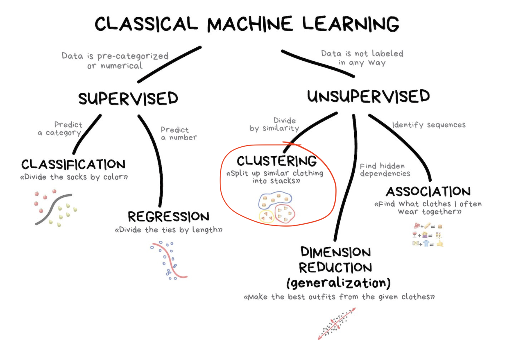
Types of Unsupervised Learning

Unsupervised learning is utilized for three main tasks [1]:

1. clustering
2. dimensionality reduction
3. association

This lecture will focus on two clustering algorithms: Hierarchical Clustering and K-means Clustering

• association rule is a rule-based method for finding relationships between variables in a given dataset.
• eg. “Customers Who Bought This Item Also Bought”, Spotify’s “Discover Weekly” playlist.
• Dimensional reduction is commonly used in the preprocessing state. It makes the data set more managable when the dimensions is too high, can combat overfitting and sometimes improve performance (eg get rid of noisy variables)

• last lecture we started talking about distance measures

• why? a lot unsupervised methods are based on distance measures

Clustering

The goal of clustering is to find groups (or clusters) such that all observations are

• more similar to observations inside their group and
• more dissimilar to observations in other groups.

Types of clustering algorithms include:

• Hierarchical
• Partitioning (e.g. k-means “hard” clustering)
• Probabilistic Clustering (e.g. Finite Mixture models)

Clustering refers to a very broad set of techniques for finding subgroups, or clusters, in a data set.

• the unsupervised version of classification
• Partitioning stipulates a data point can exist only in one cluster.
• within group similarity is maximized
• mixture models (last lecture?)

Old Faithful

Old Faithful Geyser Data is available in R (see ?faithful) and contains the following information for the Old Faithful geyser in Yellowstone National Park, Wyoming, USA.

• waiting the waiting time between eruptions and
• eruptions the duration of the eruption

Old Faithful Plot

While there are no true “classes” in this data set, many would argue that there are two natural “clusters”.

• As always PLOT!
• longer build-up of pressure implies longer eruption time
• No “true groups”
• Natural clustering
• the points in between are up for debate (with no correct answer)

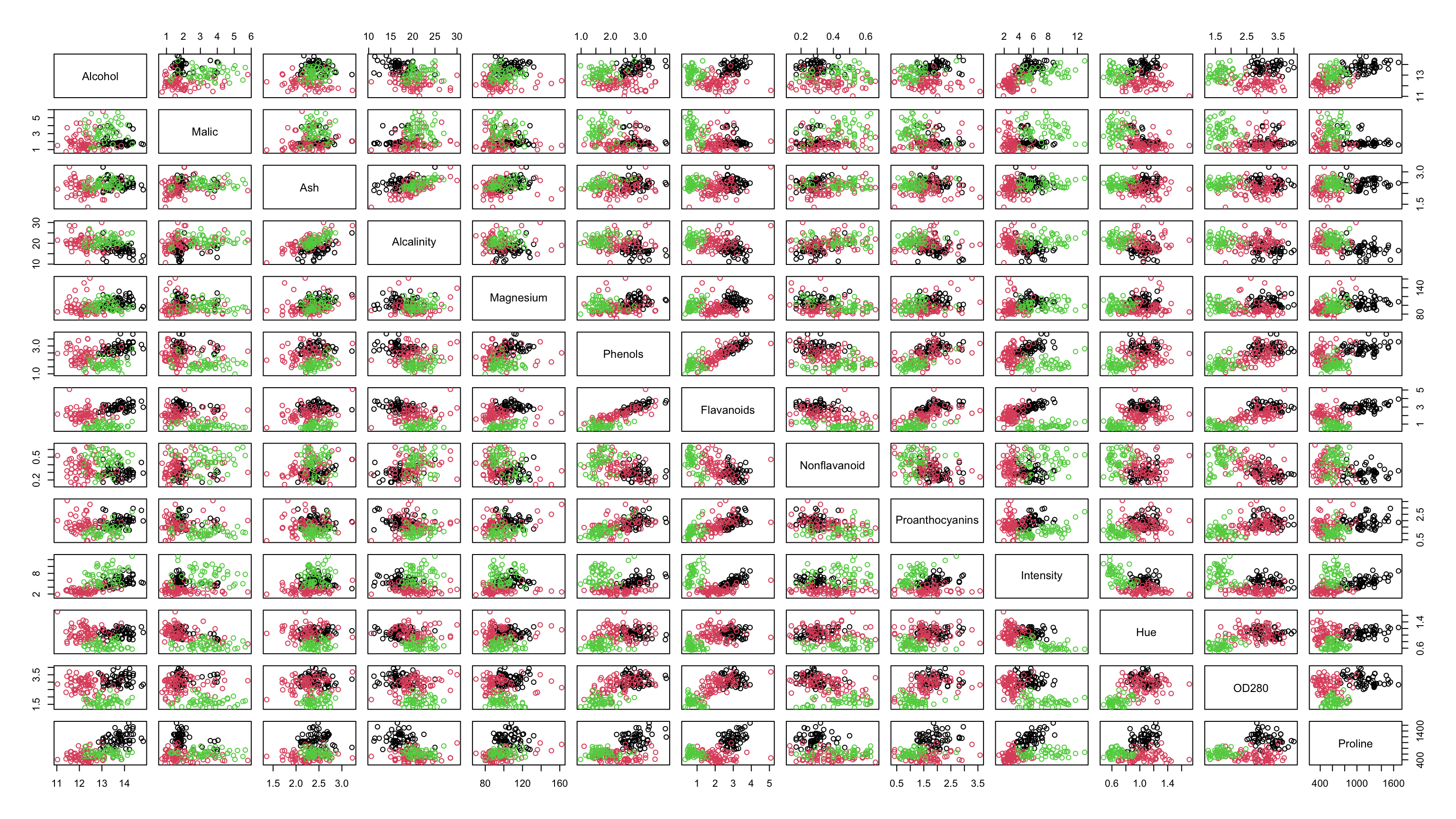
Wine

• The wine data from the gclus package comprise 178 Italian wines from three different cultivars that correspond to the wine varietals: Barolo, Grignolino, Barbera

• Recorded are 13 measurements (eg. alcohol content, malic acid, ash, …)

• there are multiple versions of this data set
• we may have seen this data before? can’t remember

• Notably, this data set does have a known class!

why should we use this for unsupervised learning?

• However, is often used to test and compare the performance of various classification algorithms.

• This an iris and crabs are example of benchmark datasets that are often used for testing an unsupervised method. Hide all the \(y\)s and use some of the metrics from the classification setting.

• these won’t be possible for genuine clustering problems

Wine Data

library(gclus); data(wine); head(wine)

Class: There are 3 classes: Barolo, Grignolino, Barbera.

multiclass and multi-dim its hard to see the separation between groups.

Comments before we begin

• Clustering will have an element of subjectivity (some may argue that there are 3 groups in the Old Faithful data set)

• It can therefore be hard to assess the results obtained from unsupervised learning methods

• For these reasons, clustering algorithms are often tried and tested on data sets for which classes do exist (eg. wine)

• crabs group by species? orange/blue? female/male, both?

• In practice unsupervised learning is often performed as part of an exploratory data analysis

EDA to uncover underlying structures, groupings, anomalies, or associations within the data, which, in turn, aids in formulating hypotheses and refining the research direction.

Hierarchical Clustering

• Once we have information on the distances between all observations in our data set, we’re ready to come up with ways to group those observations.

• Hierarchical clustering (HC), or hierarchical cluster analysis (HCA), is in many ways the most straightforward method for finding groups.

• As it’s name suggests, this method builds a hierarchy of clusters.

• by default it will use Euclidean (aka “squared distance”) but you can use whatever you like
• rather than \(k\)-means where you have to specify k this will give us all possible groups from 1 – n

Types of HC

HC can be categorized in two ways (we’ll focus on 1.):

1. Agglomerative “bottom-up” approach: each observation starts in its own cluster, and pairs of clusters are merged as one moves up the hierarchy.

2. Divisive “top-down” approach: all observations start in one cluster, and splits are performed recursively as one moves down the hierarchy.

agglomerate is far more popular and we won’t cover top-down

Agglomerative HC algorithm

Agglomerative HC can be boiled down to the following steps:

1. Start with all observations in their own groups ( \(n\) unique groups)

2. Join the two closest observations (now there are \(n-1\) groups)

3. Recalculate distances (more on this soon)

4. Repeat 2) and 3) until you are left with only 1 group.

Simple Example

Code

a <- c(1,2)
b <- c(2,2.5)
c <- c(1.5, 2)
d <- c(5,3)
e <- c(4.5,4)
x <- rbind(a,b,c,d,e)
colors <- c("purple",
 "dodgerblue",
 "firebrick",
 "forestgreen",
 "gold")
par(mar = c(4, 4, 1.5, 0.1))
plot(x, xlab="", ylab="", pch=letters[1:5], cex=2
     , ylim=c(1,5), xlim=c(0,6))

If I were to ask you to group this data, what would you do?

(Again, since we are in the realm of clustering there is no “right” or “wrong” answer).

Now let’s see what HCA produces …

• usually the have 2 groups: {a,c,b}, {e,d}
• sometimes three {a,c,b}, {e}, {d}

Step 1

Example distance matrix:

x <- rbind(a,b,c,d,e); dist(x)

	a	b	c	d	e
a	0
b	1.118	0
c	0.5	0.707	0
d	4.123	3.041	3.64	0
e	4.031	2.915	3.606	1.118	0

dist() performs method = “euclidean” by default

Jump to dendrogram

Step 2

Since a and c are the closest, we join them to a group

	a	b	c	d	e
a	0
b	1.118	0
c	0.5	0.707	0
d	4.123	3.041	3.64	0
e	4.031	2.915	3.606	1.118	0

now we need to recalculate distances

Jump to dendrogram

Step 3: Recalculating Distances

• Now that we’ve joined the two closest observations how do we determine the distance between groups?

• For instance, whats the distance between the purple group containing observations a and c and the blue group containing a single observation b? (denote this \(d_{\{ac\}\{b\}}\))

• There are 3 common ways of recalculating distances between groups; these are referred to as linkages

Jump to dendrogram

Linkages

1. Single linkage: calculates the minimum distance between two points in each cluster.

2. Complete linkage: calculates the maximum distance between two points in each cluster.

3. Average linkage: calculates the average pairwise distance between the observations inside group with those outside.

4. Centroid Linkage: calculates the distance between the centroids (mean points) of two clusters.

1. tends to produce long, elongated clusters and can be sensitive to noise and outliers.
2. often leads to compact, spherical clusters and is less sensitive to outliers compared to single linkage.
3. Average linkage tends to produce balanced, medium-sized clusters.
4. It can lead to well-balanced clusters, but it is sensitive to outliers and can result in clusters with different shapes.

Note: there are more linkage options but these are the most popular

Linkages Example:

1. Single linkage: \(d_{\{ac\}\{b\}}=d_{cb}\)
2. Complete linkage: \(d_{\{ac\}\{b\}}=d_{ab}\).
3. Average linkage: \(d_{\{ac\}\{b\}}=\frac{d_{ab}+d_{cb}}{2}\).

• single the two closest observations are c and b
• complete the two farthest observations are a and b
• average distance between a and b + distance between b and c divided by 2 (the number of pairwise distances)

Linkages Example:

	a	b	c	d	e
a	0
b	1.118	0
c	0.5	0.707	0
d	4.123	3.041	3.64	0
e	4.031	2.915	3.606	1.118	0

1. Single linkage: \[d_{\{ac\}\{b\}}=d_{cb} = 0.707\]
2. Complete linkage: \[d_{\{ac\}\{b\}}=d_{ab} = 1.118\]
3. Average linkage: \[d_{\{ac\}\{b\}}=\frac{d_{ab}+d_{cb}}{2}= 0.9125\]

notice that each linkage gives us a different value for the distance between these two clusters

Distance recalculation

	ac	b	d	e
ac	0
b	0.707	0
d	3.64	3.041	0
e	3.606	2.915	1.118	0

1. Single linkage: \[d_{\{ac\}\{b\}}=d_{cb} = 0.707\]

Adopting single linkage, our distance matrix would then get updated to something like what you see on the left.

Step 4a

Since group {a,c} and {b} are the closest, we merge them.

	ac	b	d	e
ac	0
b	0.707	0
d	3.64	3.041	0
e	3.606	2.915	1.118	0

Jump to dendrogram

Step 4b

Recalculate distance:

	abc	d	e
abc	0
d	3.041	0
e	2.915	1.118	0

now what would we merge?

Jump to dendrogram

Step 4c

Since group {e} and {d} are the closest, we merge them.

	abc	d	e
abc	0
d	3.041	0
e	2.915	1.118	0

Jump to dendrogram

Step 4d

Recalculate Distance

	abc	de
abc	0
de	2.915	0

overkill since we know there is only one choice but we can find the distance between these two clusters using single linkage

Jump to dendrogram

Step 4e

Join the two remaining groups: {a,b,c} and {e,d}

	abc	de
abc	0
de	2.915	0

Jump to dendrogram

Hierarchy of Clusters

• What we’ve done is provided a hierarchy of potential solutions to the following non-trivial questions:

  • how many groups are in this data?
  • what do they look like?

• Also, do we really need to go through the algorithm step-by-step to see the process?

Hierarchical Clustering

• We can summarize the algorithm graphically, using what’s called a dendrogram¹, i.e. a diagram representing a tree.

• On the Y-axis, “Height”, is a measure of closeness of either individual data points or clusters.

• Horizontal bars indicate the distance at which two clusters are joined.

• Large “jumps” between combining groups signify large distances between groups.

1. • we will discuss one way of seeking evidence for the number of groups.

Dendrogram

Step 1, 2, 3, 4a, 4b, 4c, 4d, 4e

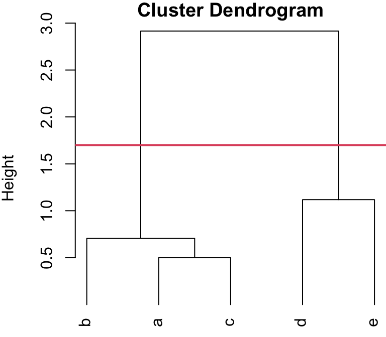
In this case, we can see that a and c are most similar, since the height of the horizontal line that joins them together is lowest on the Y-axis.

• view this as an upside down tree where the observations are the “leaves”
• a and c had a distance of 0.5 from one another so the link is plotted at a Height of 0.5.
• dist between {a,c} and {b} was 0.707
• dist between {d} and {e} was 1.118
• dist between {a,b,c} and {e, d} was 2.915

Dendrogram “jump”

In this case, the dendrogram shows us that there is big difference between cluster {a, b, c} and cluster {d, e} and that the distance within each of these clusters is pretty small.

Determining the Number of Clusters

• Dendrograms can also be used to determine how many groups are present in the data.

• We can perform a horizontal “cut” in the tree to partitioning the data into clusters.

• So generally, we can “cut” at the largest jump in distance, and that will determine the number of groups, as well as each observation’s group membership.

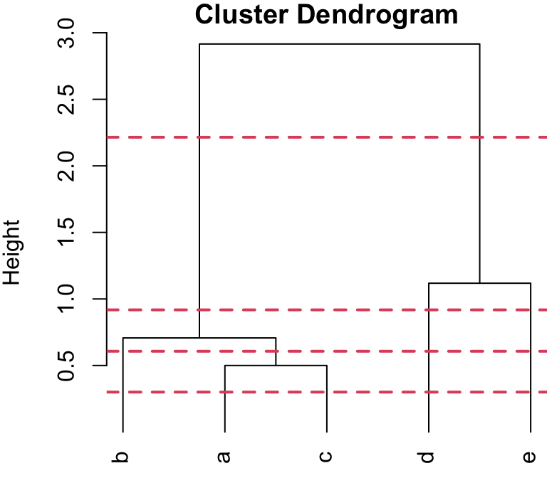
Cut-points (2 group solution)

You can visualize this as an upside-down tree (I have extended the “leaves” of the dendrogram to the the bottom to better explain the cutting process). Where you cut will dictate how many “branches” (i.e. clusters) you end up with.

usually you tell r how many groups you want it will figure out where it need to cut

Dendrogram cut at 1.7

Cutting the dendrogram somewhere along the large “jump” would result in two branches, i.e. clusters

envision having this dendrogram as a physical object and cutting it along 0.6.

2 group visualization

Which matches our intuition …

We could have cut this tree elsewhere however …

In general we will have \(n\) different partitions of the data

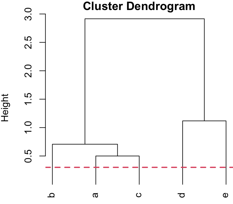
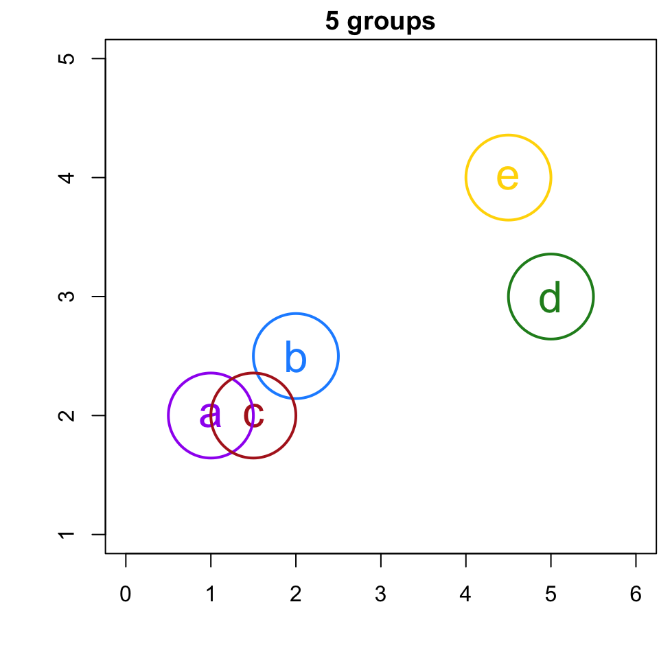
5-group solution

Any horizontal cut at r cutpts[1] or less, would result in 5 singleton clusters, i.e. 5 clusters with only 1 member.

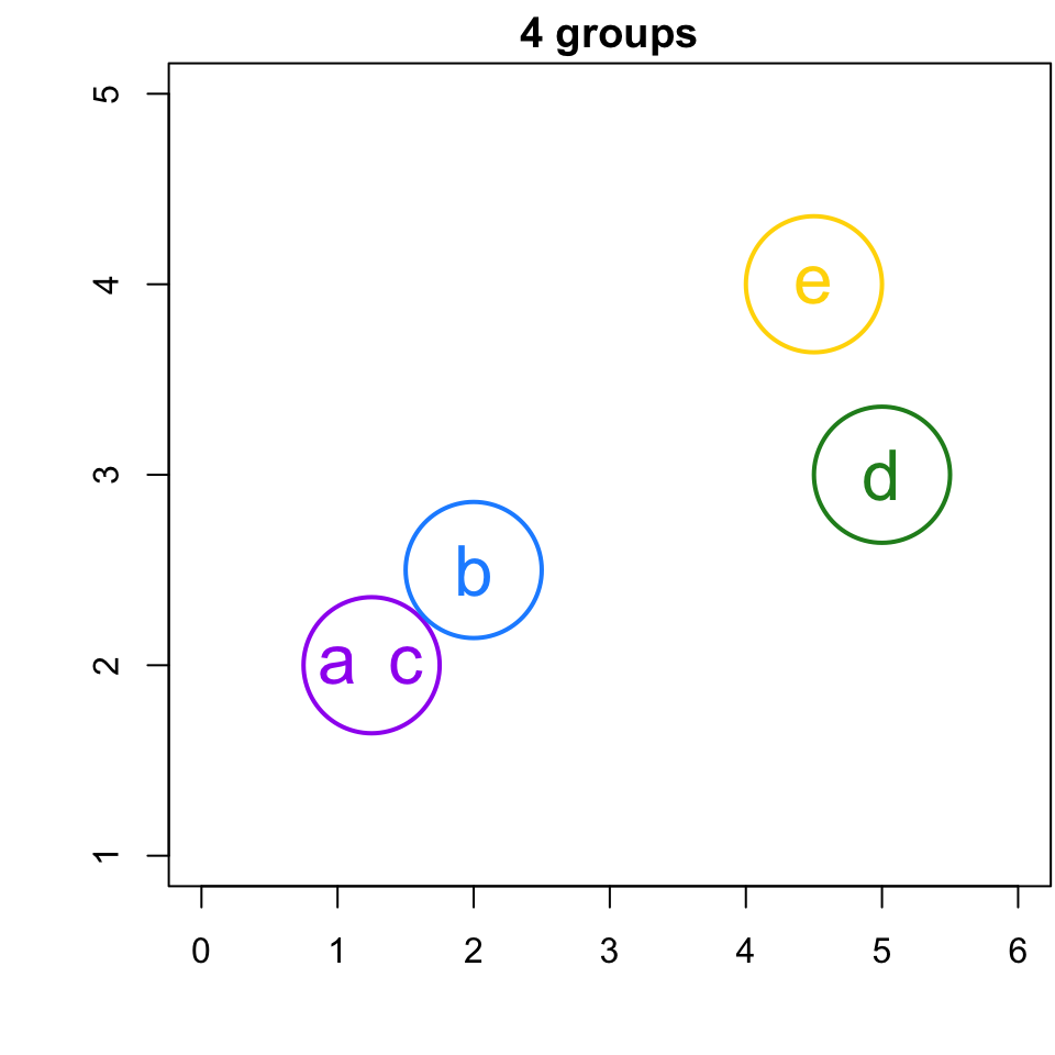
4-group solution

Any horizontal cut between r cutpts[1] and r cutpts[2] , would result in 4 clusters: {b}, {a,c}, {d}, and {e}.

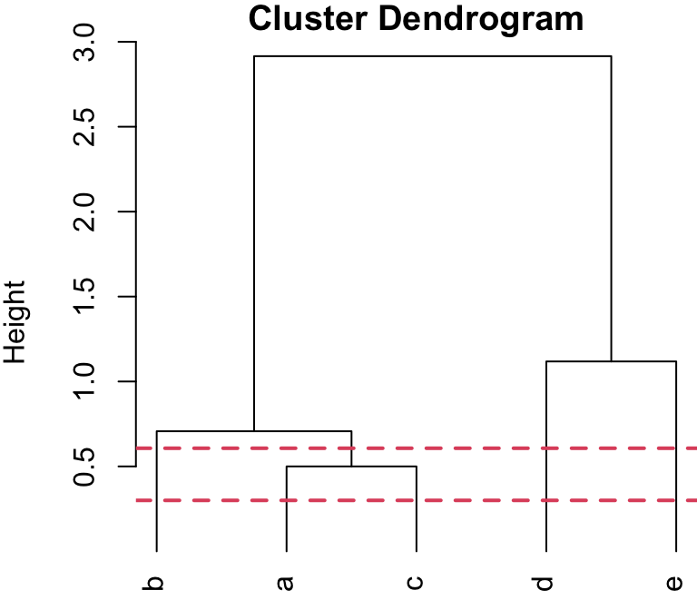
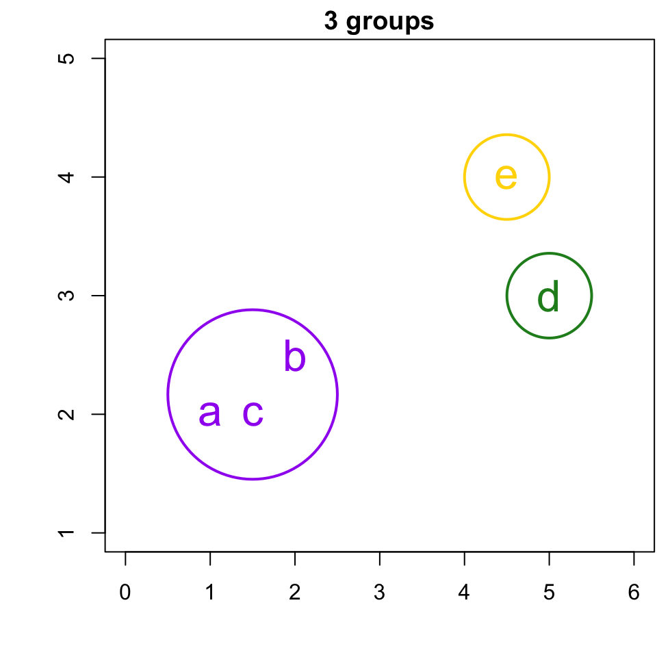
3-group solution

Any horizontal cut between r cutpts[2] and r cutpts[3] , would result in 3 clusters: {b, a,c}, {d}, and {e}.

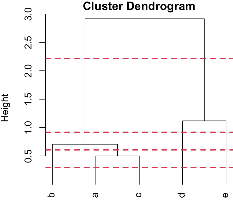
2-group solution

Any horizontal cut between r cutpts[3] and r cutpts[4] , would result in 2 clusters: {b, a,c}, {d, e}.

1-group solution

Any horizontal cut above and r cutpts[4] , would result in 1 clusters comprised of all the observations: {a,b, c, d, e}.

HC: Old Faithful

Below is the dendogram on the raw distance matrix (calculated using single linkage) on the Old faithful data

Old Faithful (2 Group Solution)

Here is the two group solution from that model:

• one singleton cluster and the rest

Old Faithful (3 Group Solution)

Here is the three group solution from that model:

• two singleton cluster and the rest

Old Faithful (4 Group Solution)

Here is the four group solution from that model:

• two singleton cluster and the 2

Question

• Hmm… These clusters are not ideal.

• What do you think might have happened?

• Can you think of something else to try?

Even though these are in the same units (minutes), perhaps we should scale the data

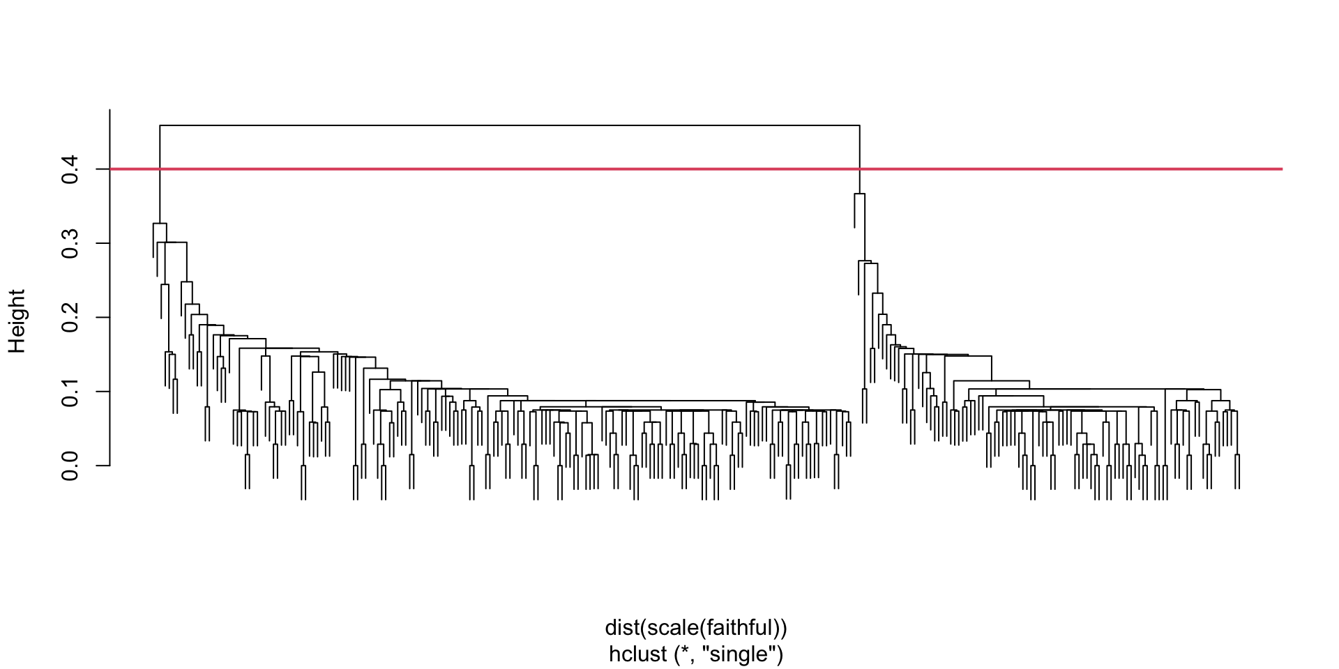
HC: Old Faithful (second attempt)

Here is the dendogram on the standardized euclidean distance matrix (using single linkage and the scale function)

faits <- hclust(dist(scale(faithful)), method="single")
plot(faits, main="", labels=FALSE)
abline(h=0.4, lwd=2, col=2)

hclust() Arguments:

• d: a dissimilarity structure as produced by dist.
  
• method: the agglomeration method to be used. This should be (an unambiguous abbreviation of) one of "ward.D", "ward.D2", "single", "complete", "average", "mcquitty", "median" or "centroid"

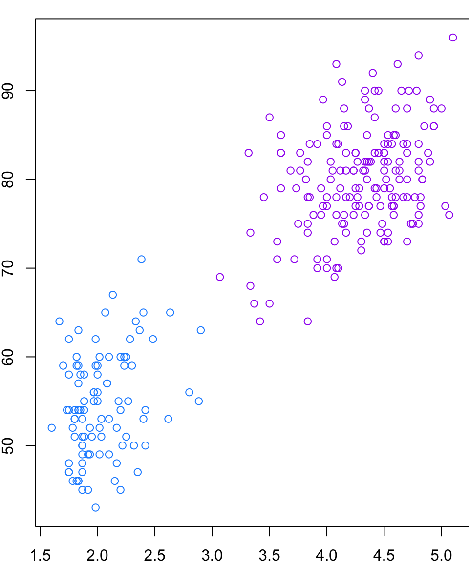
HC: Old Faithful (second attempt)

Once we perform HC on the scaled data, we get a two-group solution that much more matches our intuition …

par(mar = c(1.9, 1.9, 1, 0))     

# a vector of length n
# of clusters
cls <- cutree(faits,2)

# my colours:
mycol <- c("purple",
 "dodgerblue")

# plot the dendogram
plot(faithful,  
     col = mycol[cls])

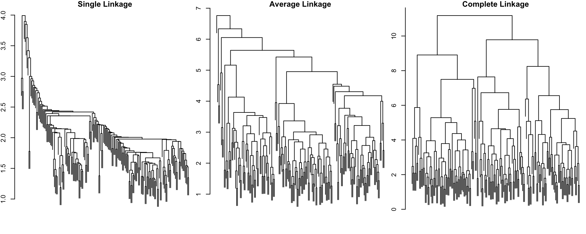
HC: Wine data

In some cases, the choice of linkage method could make a big difference. Notably, in all cases the data were scaled.

Notes on Linkage

• Single-linkage clustering is susceptible to an effect known as “chaining” whereby poorly separated, but distinct clusters are merged at an early stage

• Average linkage may lead to a number of singleton clusters (which is generally bad sign)

• Complete linkage provides a reasonable partition of the data, suggesting probably 2 or 3 groups. (We’ll come back to this later.)

• Example of chaining will be given in lab
• Dendogram well behaved for complete

Comments

Cons

• Distance matrices (of size \(n \times n\), symmetric) must be calculated.

• For very large samples, this can be time consuming (even for computers).

• Results are often sensitive to what distance type and what linkage method are used.

Pro

• easy to implement and understand

To return to the question of “what they look like”, we don’t know. We make no assumptions on the distribution of the sub-group nor do we estimate them.

The procedure is non-parametric and the only thing that you need for it is the distance measure. In the end you need to decide how to prune the tree-graph created using this procedure, so a decision about expected number of clusters needs to be made.

• although we are using numeric data, note that we can use non-numeric data as well.

K-means Clustering

Next we look at \(k\)-means Clustering.

• \(k\)-means clustering is a popular method that requires the user to provide \(k\), the number of groups they are looking for¹

• In this algorithm, each observation will belong to the cluster whose mean is closest.

After specifying the steps of the algorithm, we will demonstate on the Old Faithful data from last lecture.

• unlike hclust this requires us to tell the number of groups in advance
• it relies on Euclidean distance or other distance metrics that require numerical values to calculate the dissimilarity between data points.
• However, it is possible to use K-means with non-numeric data, but you need to convert the non-numeric data into a numerical format. Here are some common approaches to handle non-numeric data with K-means:

1. we will discuss one way of seeking evidence for the number of groups.

Algorithm

1. Randomly select \(k\) (the number of groups) points in your data. These will serve as the first centroids¹
2. Assign all observations to their closest centroid (in terms of Euclidean distance). You now have \(k\) groups.
3. Calculate the means of observations from each group; these are your new centroids.
4. Repeat 2) and 3) until nothing changes anymore (each loop is called an iteration).

• common style of clustering algorithm
• 2. assumes group labels are missing and centroids are known
• 3. assumes centroids are missing and labels are known
• The k-Means algorithm is not applicable to categorical data

1. we use “centroid” to denote the “center” of the cluster (in this case, the arithmetic mean of points belong to that cluster)

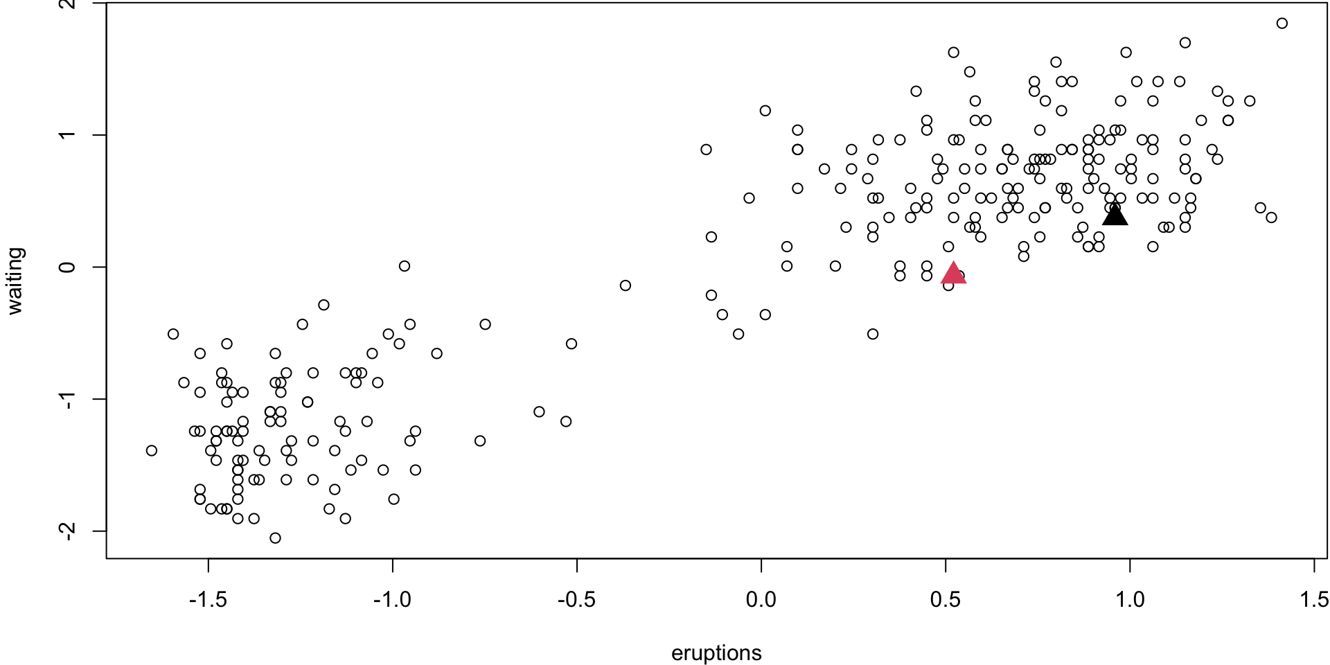
Step 1 (\(k\) = 2)

Randomly select 2 centroid

Code

par(mar = c(4, 4, 0.1, 0.1))
k=2
x <- scale(faithful)
set.seed(2021)

#1 start with k centroids
centrs <- x[sample(1:nrow(x), k),]
plot(x)
points(centrs, pch=17, cex=2, col=1:k)

Step 2

Assign obs. to their closest centroid

Code

par(mar = c(4, 4, 0.1, 0.1))
#2a) calculate distances between all x and centers
dists <- matrix(NA, nrow(x), k)
  for(i in 1:nrow(x)){
    for(j in 1:k){
      dists[i, j] <- sqrt(sum((x[i,] - centrs[j,])^2)) 
    }
  }

#2b) assign group memberships (you probably want to provide some overview of apply functions) 
membs <- apply(dists, 1, which.min)
plot(x, col=membs)  
points(centrs, pch=17, cex=2, col=1:2)

Step 3

Recalculate the means/centroids of each group.

Code

par(mar = c(4, 4, 0.1, 0.1))
#3) calculate new group centroids
oldcentrs <- centrs #save for convergence check!
for(j in 1:k){
  centrs[j,] <- colMeans(x[membs==j, ])
}
plot(x, col=membs)
points(centrs, pch=17, cex=2, col=1:2)

Step 4 (loop)

Code

par(mar = c(4, 4, 1, 0.1))
library(gifski)
count = 2
changing <- TRUE  
while(changing){
  #2a) calculate distances between all x and centers
  dists <- matrix(NA, nrow(x), k)
  #could write as a double loop, or could utilize other built in functions probably
  for(i in 1:nrow(x)){
    for(j in 1:k){
      dists[i, j] <- sqrt(sum((x[i,] - centrs[j,])^2)) 
    }
  }
  #2b) assign group memberships (you probably want to provide some overview of apply functions) 
  membs <- apply(dists, 1, which.min)
  
  #3) calculate new group centroids
  oldcentrs <- centrs #save for convergence check!
  for(j in 1:k){
    centrs[j,] <- colMeans(x[membs==j, ])
  }
  plot(x, col=membs, main=paste("Iteration", count))
  points(centrs, pch=17, cex=2, col=1:2)
  count <- count+1
  
  #4) check for convergence
  if(all(centrs==oldcentrs)){
    changing <- FALSE
    text(0.75, -1, "DONE!", cex=4)
  }
}
membs2 <- membs # save 2-group solution

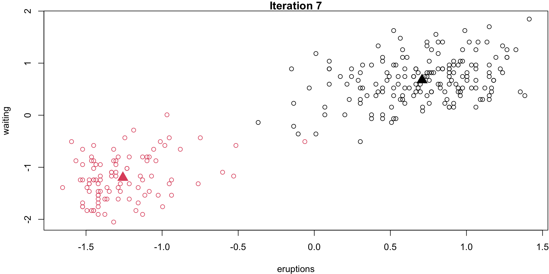
Step 4 (last iteration)

par(mar = c(4, 4, 1, 0.1))
count = 2
changing <- TRUE  
while(changing){
  #2a) calculate distances between all x and centers
  dists <- matrix(NA, nrow(x), k)
  #could write as a double loop, or could utilize other built in functions probably
  for(i in 1:nrow(x)){
    for(j in 1:k){
      dists[i, j] <- sqrt(sum((x[i,] - centrs[j,])^2)) 
    }
  }
  #2b) assign group memberships (you probably want to provide some overview of apply functions) 
  membs <- apply(dists, 1, which.min)
  
  #3) calculate new group centroids
  oldcentrs <- centrs #save for convergence check!
  for(j in 1:k){
    centrs[j,] <- colMeans(x[membs==j, ])
  }
  count <- count+1
  
  #4) check for convergence
  if(all(centrs==oldcentrs)){
    plot(x, col=membs, main=paste("Iteration", count))
    points(centrs, pch=17, cex=2, col=1:2)
    changing <- FALSE
    # text(0.75, -1, "DONE!", cex=4)
  }
}

Step 4 (last iteration)

membs2 <- membs # save 2-group solution

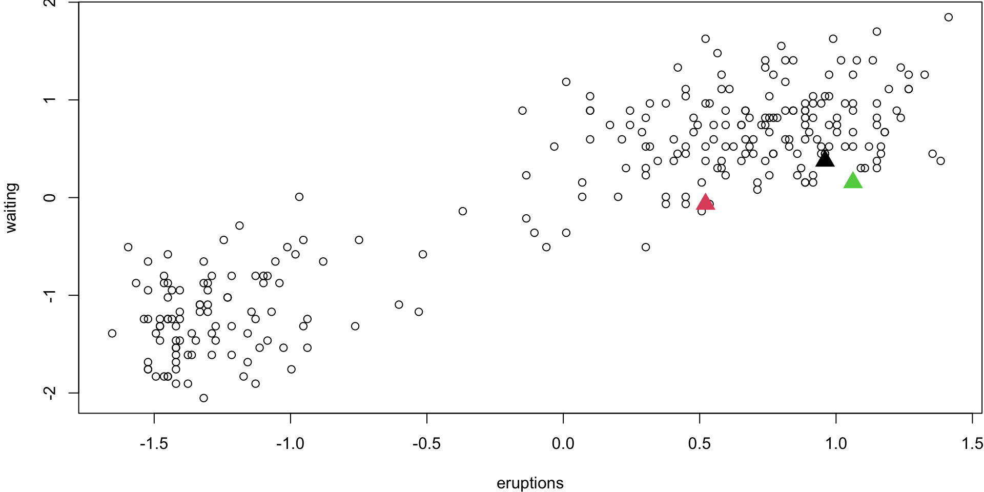
Step 1 (\(k\) = 3)

Randomly select 3 observations ( \(k\) =3). These will be your centroids for the 3 groups

Code

par(mar = c(4, 4, 0.1, 0.1))
k=3
x <- scale(faithful)
set.seed(2021)

#1 start with k centroids
centrs <- x[sample(1:nrow(x), k),]
plot(x)
points(centrs, pch=17, cex=2, col=1:k)

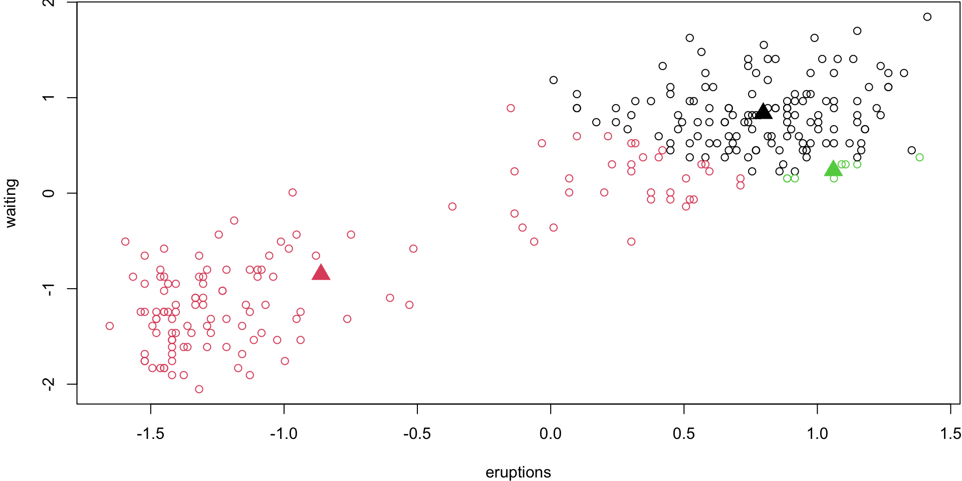
Step 2

Assign obs. to their closest centroid

Code

par(mar = c(4, 4, 0.1, 0.1))
#2a) calculate distances between all x and centers
dists <- matrix(NA, nrow(x), k)
  for(i in 1:nrow(x)){
    for(j in 1:k){
      dists[i, j] <- sqrt(sum((x[i,] - centrs[j,])^2)) 
    }
  }

#2b) assign group memberships (you probably want to provide some overview of apply functions) 
membs <- apply(dists, 1, which.min)
plot(x, col=membs)  
points(centrs, pch=17, cex=2, col=1:k)

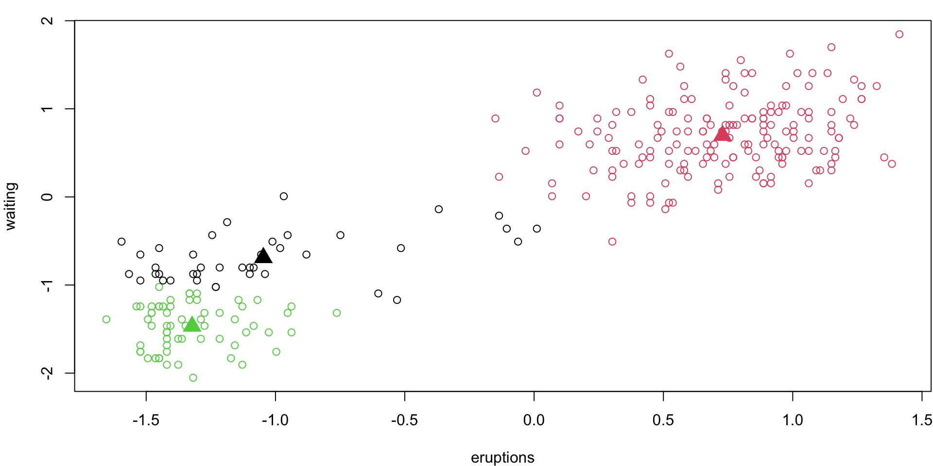
Step 3

Recalculate the means of each group. These are your new centroids.

Code

par(mar = c(4, 4, 0.1, 0.1))
#3) calculate new group centroids
oldcentrs <- centrs #save for convergence check!
for(j in 1:k){
  centrs[j,] <- colMeans(x[membs==j, ])
}
plot(x, col=membs)
points(centrs, pch=17, cex=2, col=1:k)

Step 4 (loop)

Repeat 2) and 3) until nothing changes anymore.

Code

par(mar = c(4, 4.1, 1, 0.1))
count = 2
changing <- TRUE  
while(changing){
  #2a) calculate distances between all x and centers
  dists <- matrix(NA, nrow(x), k)
  #could write as a double loop, or could utilize other built in functions probably
  for(i in 1:nrow(x)){
    for(j in 1:k){
      dists[i, j] <- sqrt(sum((x[i,] - centrs[j,])^2)) 
    }
  }
  #2b) assign group memberships (you probably want to provide some overview of apply functions) 
  membs <- apply(dists, 1, which.min)
  
  #3) calculate new group centroids
  oldcentrs <- centrs #save for convergence check!
  for(j in 1:k){
    centrs[j,] <- colMeans(x[membs==j, ])
  }
  plot(x, col=membs, main=paste("Iteration", count))
  points(centrs, pch=17, cex=2, col=1:k)
  count <- count+1
  
  #4) check for convergence
  if(all(centrs==oldcentrs)){
    changing <- FALSE
    text(0.75, -1, "DONE!", cex=4)
  }
}
membs3 <- membs # save 3-group solution

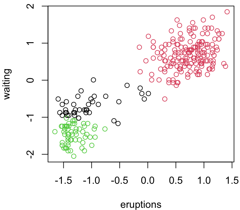
Step 4 (last iteration)

par(mar = c(4, 4.1, 1, 0.1))
count = 2
changing <- TRUE  
while(changing){
  #2a) calculate distances between all x and centers
  dists <- matrix(NA, nrow(x), k)
  #could write as a double loop, or could utilize other built in functions probably
  for(i in 1:nrow(x)){
    for(j in 1:k){
      dists[i, j] <- sqrt(sum((x[i,] - centrs[j,])^2)) 
    }
  }
  #2b) assign group memberships (you probably want to provide some overview of apply functions) 
  membs <- apply(dists, 1, which.min)
  
  #3) calculate new group centroids
  oldcentrs <- centrs #save for convergence check!
  for(j in 1:k){
    centrs[j,] <- colMeans(x[membs==j, ])
  }
  count <- count+1
  
  #4) check for convergence
  if(all(centrs==oldcentrs)){
    plot(x, col=membs, main=paste("Iteration", count))
    points(centrs, pch=17, cex=2, col=1:k)
    changing <- FALSE
    # text(0.75, -1, "DONE!", cex=4)
  }
}

Step 4 (last iteration)

membs3 <- membs # save 3-group solution

Different 3-group (loop)

Let’s do the 3-group \(k\)-means again:

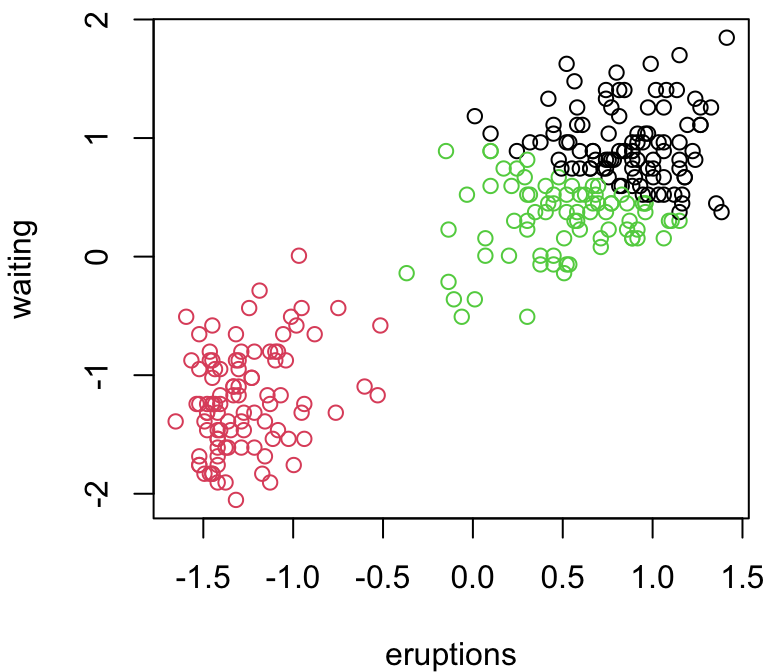
Different 3-group solution

(Last Iteration)

Code

par(mar = c(4, 4, 1.1, 0.1))
set.seed(1234)
#1 start with k centroids
centrs <- x[sample(1:nrow(x), k),]
#start loop
changing <- TRUE  
while(changing){
  #2a) calculate distances between all x and centers
  dists <- matrix(NA, nrow(x), k)
  #could write as a double loop, or could utilize other built in functions probably
  for(i in 1:nrow(x)){
    for(j in 1:k){
      dists[i, j] <- sqrt(sum((x[i,] - centrs[j,])^2)) 
    }
  }
  #2b) assign group memberships (you probably want to provide some overview of apply functions) 
  membs <- apply(dists, 1, which.min)
  
  #3) calculate new group centroids
  oldcentrs <- centrs #save for convergence check!
  for(j in 1:k){
    centrs[j,] <- colMeans(x[membs==j, ])
  }
  # readline(prompt="Press [enter] to continue")
  
  #4) check for convergence
  if(all(centrs==oldcentrs)){
    plot(x, col=membs)
    points(centrs, pch=17, cex=2, col=1:k)
    changing <- FALSE
    #text(mean(x), -1, "DONE!", cex=4)
  }
}

Code

membs3b <- membs

3 group comparison

Depending on our random starting points, we can get very different answers …

Why does \(k\)-means work?

1. Randomly select \(k\) (the number of groups) points in your data. These will serve as the first centroids
2. Assign all observations to their closest centroid (in terms of Euclidean distance). You now have \(k\) groups.
3. Calculate the means of observations from each group; these are your new centroids.
4. Repeat 2) and 3) until nothing changes anymore

2. and 3. are recursively finding the minimum within-group sum of squared distances between points and their centroids.

In other words: it minimizes within group sum of squares

Comments

Pros

• Computationally efficient, even for large data sets.
• Only \(n \times k\) distance matrices needed
• Relatively straightforward
• Often provides clearer groups than HC.

Cons

• stochastic, i.e. random (as opposed to deterministic)
• can return local optimal rather than global
• not for categorical \(X\)
• Groups will be found no matter what.

notes

Pros

• fast to run
• (distances between $n$ observations and $k$ centroids).

Cons - global will find the best solution no matter what but they are very expensive - we’ll do a bunch of random starts and compare - groups no matter what even if there are no groups present in the data. - not applicable to categorical since it relies on euclidean

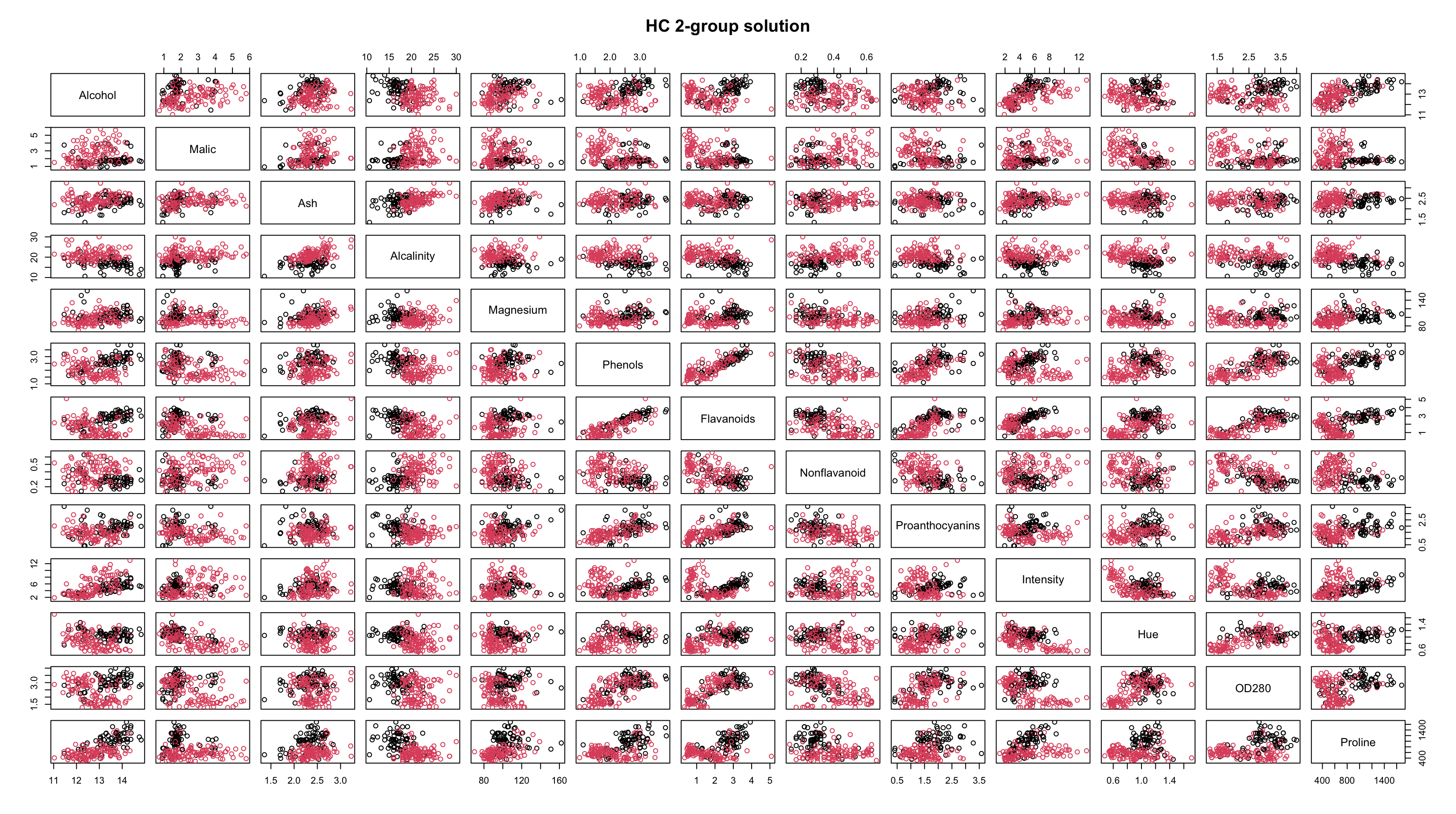
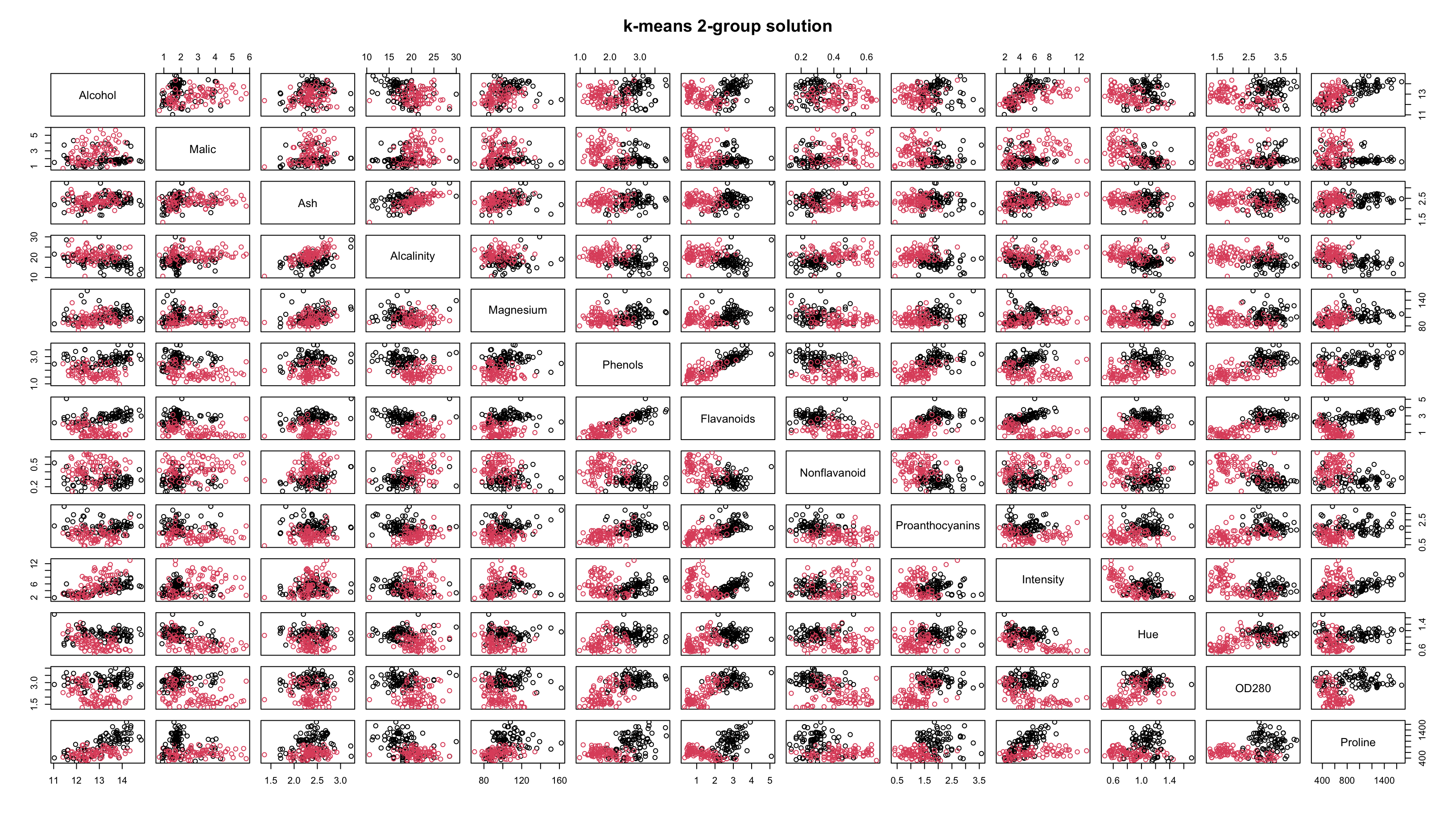
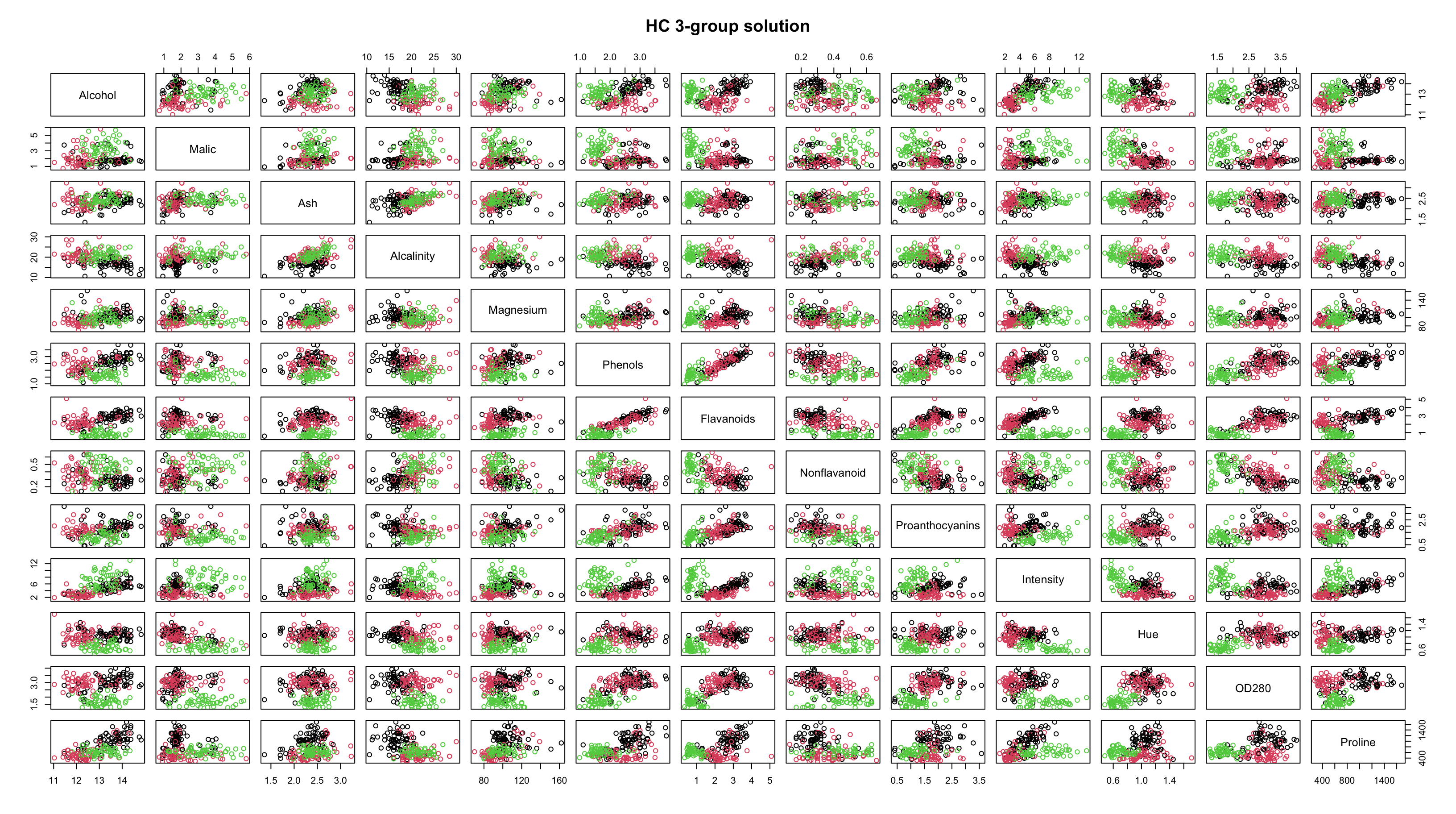
Wine

• Let’s return to the wine data set

• Let’s apply HC and \(k\)-means and then investigate the results…

• Recall that complete linkage appeared to be the most appropriate linkage choice and it suggested 2 or 3 groups.

• k-means, using a pre-specified number of clusters
• In hierarchical clustering one can stop at any number of clusters (find appropriate one from dendrogram)
• k-means (random) HC (deterministic)

Code

par(mar=c(0,4,1,0))
library(gclus)
data(wine)
wc <- hclust(dist(scale(wine[,-1])),method="complete")
w2 <- cutree(wc,2)
w3 <- cutree(wc,3)
# abline(h=1, col=2, lwd=2)
plot(wc, main= "Complete Linkage", labels=FALSE)

Code

set.seed(13)
wk3 <- kmeans(scale(wine[,-1]),3,nstart=25)
par(mar = c(3.9, 3.9, 1, 1))  
pairs(wine[,-1], col=wk3$clus, main = "k-means 3-group solution")

Comparing Results

• By looking at the plots, it seems as though the results are pretty similar between \(k\)-means and HC.

• The resolution makes it tough to tell, but the solutions are not identical.

• Both methods are finding most of the group structure, but…

  • \(k\)-means only misclassifies 6 of the 178 wines
  • whereas HC misclassifies 29 of them

notice that the class mapping seems to have been switched here… it looks the green and red group labels have been swapped for kmeans and HC

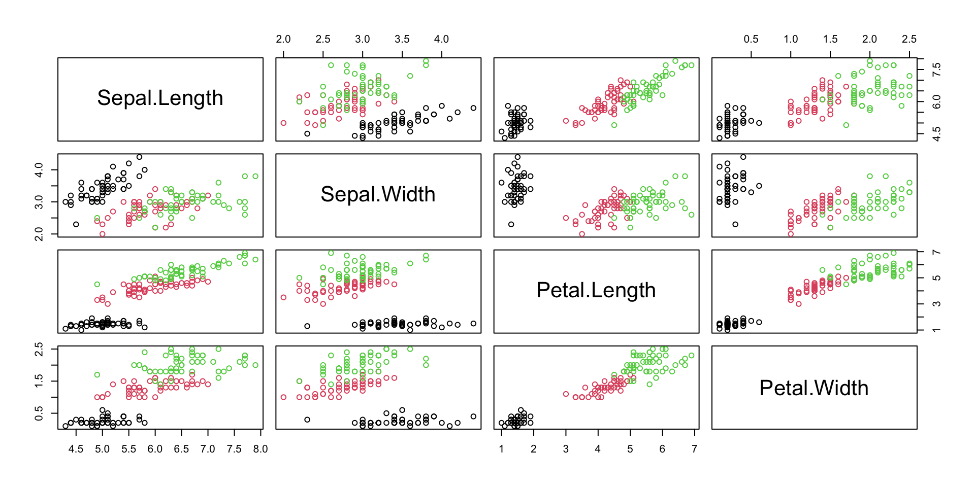
Assessing Results

• But remember, we actually have know classes (but hid them in training)

• The wine data set among others (e.g. Iris, crabs) are benchmark data clustering data sets that are used to assess performance

• With the understanding that we wouldn’t be able to do this is a authentic clustering problem, in these scenarios we would be able to build confusions matrices and calcaulte classification error, etc.

• barolo is more expensive (food authenticity problem)

Confusion Matrices

wineknown <- c("Barolo","Grignolino","Barbera")[wine[,1]]
ktab <- table(wineknown,wk3$clus)
htab <- table(wineknown,w3)

HC

library(kableExtra)

htab %>%
  kable(booktabs = T) %>%
  kable_styling()

	1	2	3
Barbera	0	0	48
Barolo	51	8	0
Grignolino	18	50	3

\(k\)-means

ktab %>%
  kable(booktabs = T) %>%
  kable_styling()

	1	2	3
Barbera	0	48	0
Barolo	59	0	0
Grignolino	3	3	65

Notice how the correctly labeled observations do not necessarily fall on the main diagonal!

Partitioning and Hierarchical

• Neither HC or \(k\)-means can really be considered “statistical” in the sense of:

  • What model are we assuming?
  • How can we test whether the model is accurate?

• They are basically ad hoc methods that mostly follow from intuition and tend to perform alright.

• Eventually, we’ll see clustering via mixture models; the unsupervised equivalent of discriminant analysis.

goodness of fit test (even if we don’t have the truth)

Dealing with Random Starts

• As mentioned, \(k\)-means minimizes the within group sum of squares (WSS); however, it does so locally (not globally)

• Furthermore, since it’s initialized randomly, results change from run to run.

• Importantly: it’s fast! So we can run it many times, and choose the solution with the smallest within-group sum of squares for those runs.

• In fact, there’s a built in argument in R…

Iris

• This famous (Fisher’s or Anderson’s) iris data set gives the measurements in centimeters of the following four variables:

  • sepal length and width
  • petal length and width,

• Data set contains the measurements on 50 flowers from each of 3 species of iris.

• The species are Iris setosa, versicolor, and virginica.

Iris plot

par(mar = c(3.9, 3.9, 0, 1))  
plot(iris[,-5], col=iris[,5])

Demo 1

set.seed(1)
kiris <- kmeans(iris[,-5], 3)
table(iris[,5], 
      kiris$cluster)

            
              1  2  3
  setosa      0  0 50
  versicolor 48  2  0
  virginica  14 36  0

set.seed(2)
kiris <- kmeans(iris[,-5], 3)
table(iris[,5], 
      kiris$cluster)

            
              1  2  3
  setosa      0 50  0
  versicolor 48  0  2
  virginica  14  0 36

These are the same solution but with swapped labels

Demo 2

set.seed(3)
kiris <- kmeans(iris[,-5], 3)
table(iris[,5], 
      kiris$cluster)

            
              1  2  3
  setosa     33  0 17
  versicolor  0 46  4
  virginica   0 50  0

set.seed(4)
kiris <- kmeans(iris[,-5], 3)
table(iris[,5], 
      kiris$cluster)

            
              1  2  3
  setosa      0  0 50
  versicolor 48  2  0
  virginica  14 36  0

These are not the same solution

Demo 3

ix <- iris[,-5]
class <- iris[,5]
ko <- kmeans(ix, 3, nstart=25)
table(class, ko$cluster)

            
class         1  2  3
  setosa      0  0 50
  versicolor  2 48  0
  virginica  36 14  0

If we run multiple starts, R will automatically report the solution which had the smallest within group sum of squares

Determining Number of Groups

• For hierarchical, we have an argument for the number of groups present in the data (largest jump in dendrogram).

• For \(k\)-means, we need to specify \(k\) but can still provide some guidance

• We can plot the WSS (within sum of squares) for differing numbers of groups

WSS

clustore <- matrix(0, 
        nrow=150, ncol=10)
wsstore <- NULL
x <- scale(iris[,-5])
for(i in 1:10){
  dum <- kmeans(x, i, nstart=25)
  clustore[, i] <- dum$cluster
  wsstore[i] <- dum$tot.withinss
}

plot(wsstore)

par(mar=c(4,4,1.1,0))
plot(wsstore, ylab="Within Sum of Squares", main= "Scree Plot")

We look for the “elbow” in the so-called “scree” plot.

fairly subjective As the number of clusters increases, the variance (within-group sum of squares) decreases. The elbow at five clusters represents the most parsimonious balance between mini- mizing the number of clusters and minimizing the variance within each cluster.

No groups?

Also as previously noted, \(k\)-means can seem like it finds groups, even when they may not exist.

par(mar = c(3.9, 3.9, 1, 1))  
nogroups <- cbind(rnorm(500),rnorm(500))
plot(nogroups)

k-means “solution”

K-means with \(k\) = 7 will always return a “solution”

par(mar = c(3.9, 3.9, 1, 1))  
set.seed(311)
nogk <- kmeans(scale(nogroups),7)
plot(nogroups, col= nogk$cluster)

WSS (no groups)

clustore <- matrix(0, 
        nrow=nrow(nogroups), ncol=10)
wsstore <- NULL
x <- scale(nogroups)
for(i in 1:10){
  dum <- kmeans(x, i, nstart=25)
  clustore[, i] <- dum$cluster
  wsstore[i] <- dum$tot.withinss
}

par(mar = c(3.9, 3.9, 1, 1))  

par(mar=c(4,4,1.1,0))
plot(wsstore, ylab="Within Sum of Squares", main= "Scree Plot")

As the number of clusters increases, the variance (within-group sum of squares) decreases. There is no elbow providing evidence that there is no “good” choice amongst these options.