Blogdown Cheatsheet
By R package build in Personal
July 9, 2021
Introduction
I find when creating content for my website and courses I am constantly using (and forgetting) the syntax for a relatively small collection of tasks. This blog will consolidate examples for some commonly used content on my website.
- General markdown syntax
- Cross-referencing content using hyperlinks (either to urls or pages within my own website)
- Including R content (inline or in “chunks”, R output)
- Including images
- …
This blog post is a collection of basic examples demonstrating how to do the aforementioned tasks in .Rmd or .Rmarkdown.
General Markdown Syntax
The above header was created with the syntax # General Markdown Syntax. This is called a level 1 header and it is the biggest. If you are familiar with LaTex, you might like to think of this as \section. As you increase the number of hashtags, the font size will get progressively smaller. The “level” is an indication of how many hashtags you used preceded your text with. For example:
Level 2 header
The above header was created with the syntax ## Level 2 header. If you are familiar with LaTex, you might like to think of this as \subsection.
Level 3 header
The above header was created with the syntax ### Level 3 header. If you are familiar with LaTex, you might like to think of this as \subsubsection.
Level 4 header
The above header was created with the syntax #### Level 4 header.
Level 5 header
The above header was created with the syntax ##### Level 5 header
Level 6 header
The above header was created with the syntax ###### Level 6 header. Notice that this doesn’t appear any different than the level-5 header; but you probably wouldn’t want to use a sub sub sub sub sub section anyhow! Level 6 headers
Tables
Simple table
To create a simple table in markdown:
- There must be at least 3 dashes separating each header cell.
- The outer pipes (|) are optional.
- Things don’t need to be tabbed (ie pretty)
For example, while the following is harder for a human to read, R will render it with no problems:
Markdown | Less | Pretty
--- | --- | ---
*Still* | `renders` | **nicely**
1 | 2 | 3
the above code produces:
| Markdown | Less | Pretty |
|---|---|---|
| Still | renders |
nicely |
| 1 | 2 | 3 |
Alignment
The following example was taken from this markdown cheatsheet.
Colons can be used to align columns. For example:
| Tables        | Are           | Cool          |
| ------------- |:-------------:| -------------:|
| left-aligned  | this col is   | right-aligned |
| (default)     | centered      |   $12         |
| zebra stripes | and neat      |    $1         |
Gets rendered to:
| Tables | Are | Cool |
|---|---|---|
| left-aligned | this col is | right-aligned |
| (default) | centered | $12 |
| zebra stripes | and neat | $1 |
Captioned tables
To be able to cross-reference a Markdown table, it must have a labeled caption. To do this, include Table: (\#tab:label) Caption here either at the top or bottom of your table (a single line must separate this caption and the table). Note that the label ID must have the prefix “tab:”, for e.g., tab:simple-table no simple-table.
Markdown | Less | Pretty
--- | --- | ---
*Still* | `renders` | **nicely**
1 | 2 | 3

Table: (\#tab:simple-table) Caption here
the above code produces:
| Markdown | Less | Pretty |
|---|---|---|
| Still | renders |
nicely |
| 1 | 2 | 3 |
Table: Table 1: Caption here
For some reason, when I do this, it produces the caption “Table: Table …”. When I try to remove the leading “Table:” then R studio no longer recognizes this as a Table label (and just places the verbatim text into the document). The repetition annoys me and I found a fix (or hack?) here. Come back to this to sort this out properly
I found that I had to remove the initial “Table:” and enclose my caption in an html tag for this to work: - vkehayas Mar 29 ‘19 at 9:54
<caption> (\#tab:lable) My caption </caption>
For example:
<caption> (\#tab:foo) Top caption. </caption>

| Sepal.Length| Sepal.Width| Petal.Length|
|------------:|-----------:|------------:|
|          5.1|         3.5|          1.4|
|          4.9|         3.0|          1.4|
|          4.7|         3.2|          1.3|
|          4.6|         3.1|          1.5|
| Sepal.Length | Sepal.Width | Petal.Length |
|---|---|---|
| 5.1 | 3.5 | 1.4 |
| 4.9 | 3.0 | 1.4 |
| 4.7 | 3.2 | 1.3 |
| 4.6 | 3.1 | 1.5 |
We reference this using \@ref(tab:foo) which renders to the table number. So “Table \@ref(tab:foo)” produces: “Table 2”. Clicking the table number will navigate the reader to the appropriate place in the webpage where the table lives. Since the table is right above you probably won’t see any movement in this example.
Cross-referencing
Hyperlinks to Sections
If you want to make a clickable reference (i.e. hyperlink) to the section heading, for example the “General Markdown Syntax” section, you may use \@ref(general-markdown-syntax) which gets rendered to: 2. If you would like to have text linking to the section in place of the section number, you can use the [1](2) syntax where 1 is replaced by the text you want to be clickable, and 2 is the label id. For example, [take me to section 2](general-markdown-syntax) gets rendered to:
take me to section 2.
Note that Pandoc creates default label IDs from the text associated with the header. For instance, # This is a Header Name will be automatically assigned the label id this-is-a-header-name; please note that all captial letters have been converted to lower-case. You can (and should) manually assign a unique ID to a desired labels, using the syntax {#id}. However, this doesn’t work for me for some reason. For example, in this section if I instead use:
# Cross-referencing {#crossref}
and reference the section using \@ref(crossref) it produces ??. For this reason I have removed the manual ID so that i can reference it with the default1 \@ref(cross-referencing) which renders to the section number: 3. Apparently this problem arises because Markdown itself does not support this functionality. Thankfully, I have found a good solution
here (the example they provide is copied below). To demonstrate, if I want to link to the section “Your leader” with the text “Take me to your leader” I would use
### <a id="your_leader"></a>Your leader
to create the header and
[Take me to your leader](#your_leader)
to link to it (try it here: Take me to your leader) . P.S. The above uses HTML anchor tags but you will still be able to use the default reference ID created by Pandoc. A summary of this information is provided in Table 3.
| Header code | Cross-reference | Output |
|---|---|---|
# <a id="cross_ref"></a>Cross-referencing |
[this](#cross_ref) |
this |
# <a id="cross_ref"></a>Cross-referencing |
\@ref(cross-referencing) |
3 |
## <a id="ref_to_sec"></a>Hyperlinks to Sections |
[that](#ref_to_sec) |
that |
## <a id="ref_to_sec"></a>Hyperlinks to Sections |
\@ref(hyperlinks-to-sections) |
3.1 |
Referencing Tables by number
In the above example I reference the table by a clickable number. For more on this read the section on captioning tables.
Linking to pages within website
If you want to link to content within your website, you can link to them by referencing their unique location in the site directory (see “Site structure” in my How to create a website using blogdown)
URL links
You can make reference to a webpage by simply by copying and pasting the plain http address. For example http://google.com renders to:
http://google.com. Note that this will not work if you are missing the “http://”. For example google.com renders to: google.com which is not clickable.
On a somewhat related note, you may have noticed that a link is created with the level 1, 2, and 3 headers. If you click the icon you will notice that the URL in your address bar will change. Namely the address will append /#name-of-header. This allows you to share a particular section of your webpage. For example, by sharing the link
http://irene.vrbik.ok.ubc/blog/2021-07-09-blogdown-cheatsheet/#ulr-links the receiver will be directed to this section of this blogpost as opposed to to the top of the page.
N.B. If you created your own HTML anchor to name your section header, the link will have a slightly different format. For example the
Your leader section (which used the anchor label “your_leader”) has the corresponding URL:
http://irene.vrbik.ok.ubc/blog/2021-07-09-blogdown-cheatsheet/#a-idyour_leaderayour-leader I think the general form it will take is
/#a-idanchor-idaanchor-id
but I’m not sure.
Footers
This is how you make footers. A quick brown fox2 jumped over the lazy dog3. Notice that the footnote numbers act as an id linking the text to the footnote and do not influence the order in which they appear at the end of the document. For instance, in the above text I used fox[^1] and dog[^2], however, since they are the second and third footnote used in the document, the superscript used is a “2” and a “3”. If I decided to include yet another footnote befor the appearance of this text, they would be replaced with “4” and “5”.
Including R Content
R markdown makes it really easy to embed both R input and output directly into the document. For those of you familiar with the annoyance of incorporating, for instance, R plots into LaTeX documents (which includes created the plot in R saving to file, creating a path to file, copying and pasting the source code into a Verbatim environment and redoing the above if the plot should change) will appreciate even more the ease at which R markdown files can handle this.
Inline
Inline code will appear, well in-line, with regular text. To put another way, the code will not be isolated in a standalone line or highlighted code block (for that see the R chunk section). Inline code provides a great way to incorporate a short snippet of code without breaking up the paragraph. I use them in two contexts, to execute or highlight short snippets of R code, or to create typewritter or monospaced font (usually to highlight variable/function names).
Inline typewritter (monospaced) text
To include text in monospaced font inline with regular text, simply wrap the text with single backticks ``. For example, `this` gets render to:this.
Inline R code
To include inline R code, wrap the R code in single backticks with a leading r. For example, ` r 1+3 ` gets rendered to: 4. Notice how only the output of the R code is displayed.
Blocks
Code blocks will be separated into isolated blocks. Usually these blocks will be highlighted in some way (eg a gray background with text appearing in monospaced font). These blocks provide a way of highlighting multiple lines of codes while clearly distinguishing this content from the regular written content of your document. Akin to inline code, I find myself using them in two contents: the first to highlight/execute small R programs, the second to create an environment that uses typewritter or monospaced font (how a LaTeX user might use the verbatim enviornment). The former is created using R “chunks” while the latter uses plain code blocks.
R Chunks
You also have an option of including an R “chunk”. A chunk will be a block of R code that will appear on a new line (as opposed to inline with regular text). For this, I either use the keyboard shortcut Shift + Command + I (on a Mac) or click the little icon () which populates the following into my R markdown file:
```{r}

```
The necessary R code is placed in between the leading and trailing tripple backticks. For example,
```{r}
1+3
y = 25
```
renders as
1+3
## [1] 4
y = 25
To see how to suppress in input or output read the Chunk Options section. Notice how you can reference objects in inline text. For example ` r y ` will render to: 25
Plain code blocks
Occasionally I would just like verbatim monospaced text. For this, I use the R chunk method as described above and simply remove the {r} bit from it. In other words, wrap your verbatim text in three leading and trailing backticks.
This is not R code
To created the verbatim R chunks with the {r} bit, you need to use the trick as described in the
bookdown section 5.6:. That is, we need to include `r ''` in the chunk header.
Quotes
You can create indented quotes by placing the text on lines beginning with >. For instance,
> This is a
> quote
gets rendered to:
This is a quote
Chunk options
Chunk options are separated by commans in the chunk header (i.e. in between the curly brackets). For example:
{r, label="chunk-label", results='hide', fig.height=4}
{r, chunk-label, results='hide', fig.height=4}
My go-to resource for code chunks is Yihui Xie’s webpage. Another resourece is R Studio lesson 3. I have summarized some useful options below:
echoifTRUEthe source code will be displayed in the document, otherwise it will be suppressedevalifTRUEthe code will be evaluated; you can specify particual lines to be evaluated as well ( more here)labela unique label which can be used for plot labelling and referencing throughout the document. If not specified, a generic label will be given, egunnamed-chunk-i. Chunk label’s should only use alphanumeric characters (a-z, A-Z, 0-9), slashes (/), or dashes (-), i.e. no underscoreswarningifFALSEwarnings will be suppressedincludeifFALSEthe code output will be suppressed (note that the code will still be evaluated)tidyifTRUEcode will be reformatted to look prettier (eg overflow text will be wrapped)sizedetermines font size. Options are borrowed from Latex: tiny, scriptsize, footnotesize, small, normalsize, large, Large, LARGE, huge, Hugebackgroundcode background colour (default gray: ‘#F7F7F7’)cacheifTRUEobjects created by the corresponding chunks are saved and skipped when recompiling the document (unless the chunk has been modified). This is helpful when the code takes a long time to run.resultsthis is something I don’t fully grasp yet but it seems relevant
Some plot specific chunk options are:
fig.pathname of subdirectory to store generated figures (default ‘figure/’)fig.showdefault `asis’. Describes how to show/arrange the plots. Options:asis: Place plots exactly where they were generatedhold: output plots at the end of a code chunk.animate: Concatenate all plots into an animation if there are multiple plots in a chunk ( more on animation)hide: Generate plot (and save tofig.path) but hide them in the output document.
dev: the generated extension to the figure (‘pdf’ for LaTeX output and ‘png’ for HTML/Markdown)fig.width,fig.height: Width and height of the plot (in inches) (default is 7 for both)out.width,out.height: how plots are scaled. For example:.8\\linewidth,3in, or8cm(for LaTeX output);300px(for HTML)\\maxwidth(default for .Rnw)- as a percentage of the linewidth. eg
40%=0.4\linewidth
fig.alignoptions:default,left,right, andcenter.fig.capa figure caption
To change the default settings, you may specify chunk values using knitr::opts_chunk$set(). For example, I will often specify a figure height in the following way:
```{r, setup, include=FALSE}
knitr::opts_chunk$set(
  comment = '', fig.width = 6, fig.height = 6
)
```
Panelsets
There is a nifty way to present your output/source code that uses panelsets. I found the code for this by sourcing the files used to create this page. I have found documentation regarding panelsets used in xaringan slides ( slides, slide code NHS-R), but haven’t found any documentation about their use in markdown files. But they are cool.!
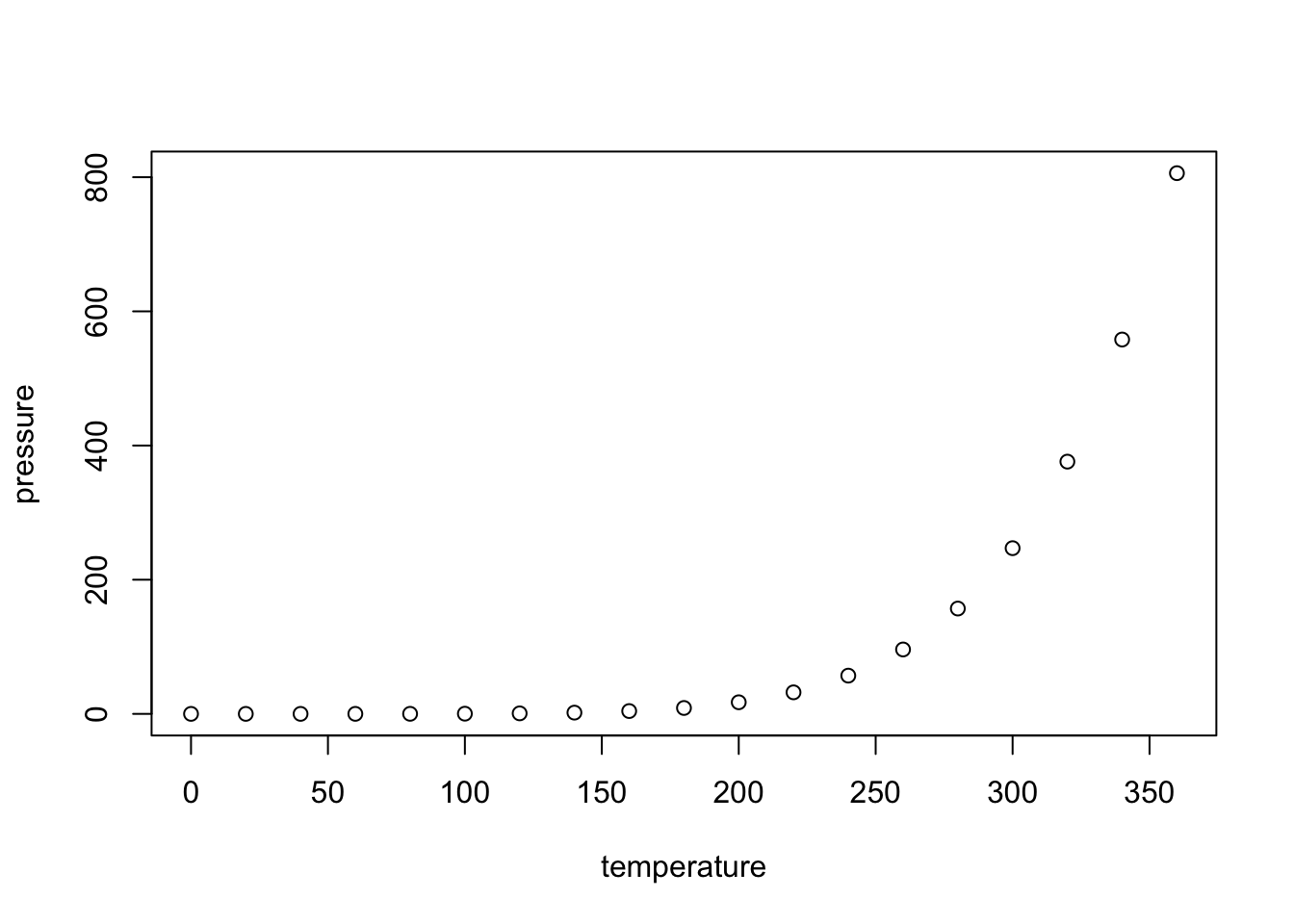
plot(pressure)
Your leader
This is used for demonstrational purposes in the cross-referencing section.
Including Images
With blogdown you can include images produced by R, as well as saved images (in the form of .png for example).
Including Saved Images
The general syntax for including static images is:

Where My picture is a caption and /path/to/image.png references the location of the file. Please note the leading slash! (without it, the path will be relative). In a blogdown site, this image file is assumed to be located in the /static/ directory. So if you save your image file in a subdirectory called /static/images/, the file path would be (/images/image.png).
While I think there may be a way you can save your images within the directory in which your Rmd file lives, Yihui recommends storing images in the static/ folder [
1]4. Take this example from
2.7 of the blogdown book:
An image
static/foo/bar.pngcan be embedded in your post using the Markdown syntax. The link of the image depends on yourbaseurlsetting inconfig.toml. If it does not contain a subpath,/foo/bar.pngwill be the link of the image, otherwise you may have to adjust it, e.g., forbaseurl = "http://example.com/subpath/", the link to the image should be/subpath/foo/bar.png︎
In one of Yihuyi’s R conference talks (I can’t remember which one) I recall him mentioning that he usually saves his images to the web and links to them with their URL. To do this, simply replace the image path to a URL in quotes:

You can also use the knitr::include_graphics function to include images in an R chunk. This has the added benefit of the code chunk options. As with the above markdown syntax, this function works with either URLs or file paths; however, file paths need to be wrapped in quotations. The below example uses out.width='20%' to scale the images down a bit:
url <- 'https://rmarkdown.rstudio.com/docs/reference/figures/logo.png'
knitr::include_graphics(rep(url, 3))
Figure 1: Three knitr logos included in the document from an external PNG image file.
knitr::include_graphics(rep(url, 2))
Figure 2: Why does it repeat here
Figure 3: Why does it repeat here
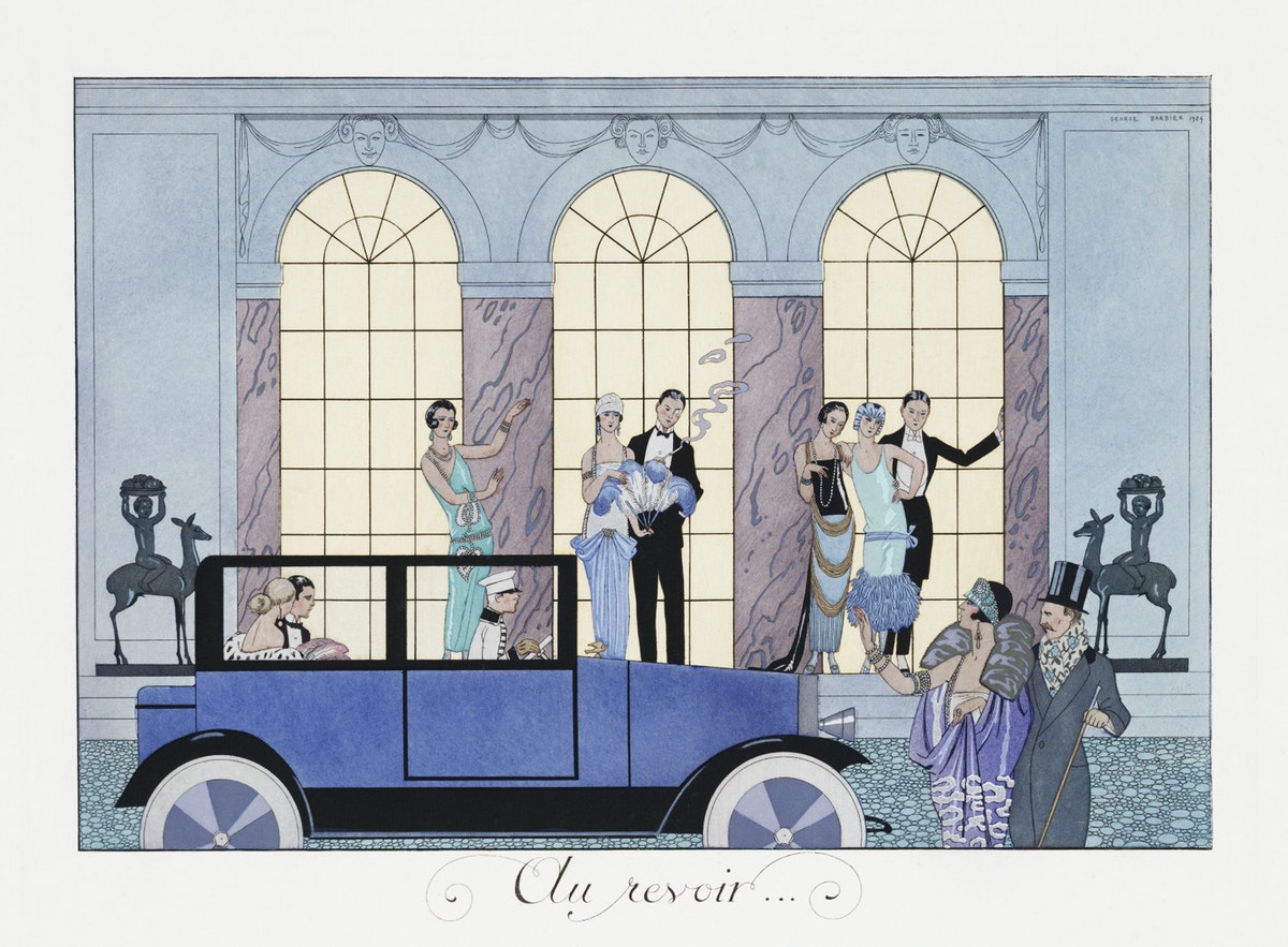
When using knitr::include_graphics with a image file located in static, I could not have it run without specifying error = FALSE (a solution I read about
here)
knitr::include_graphics("/img/revoir.jpg", error=FALSE)
Including Images Generated With R
To embed an image produced using R, simple copy and paste the source code into an R chunk. For example:
```{r simple-plot, fig.cap="What a simple plot"}
plot(1:10)
```
produces the following:
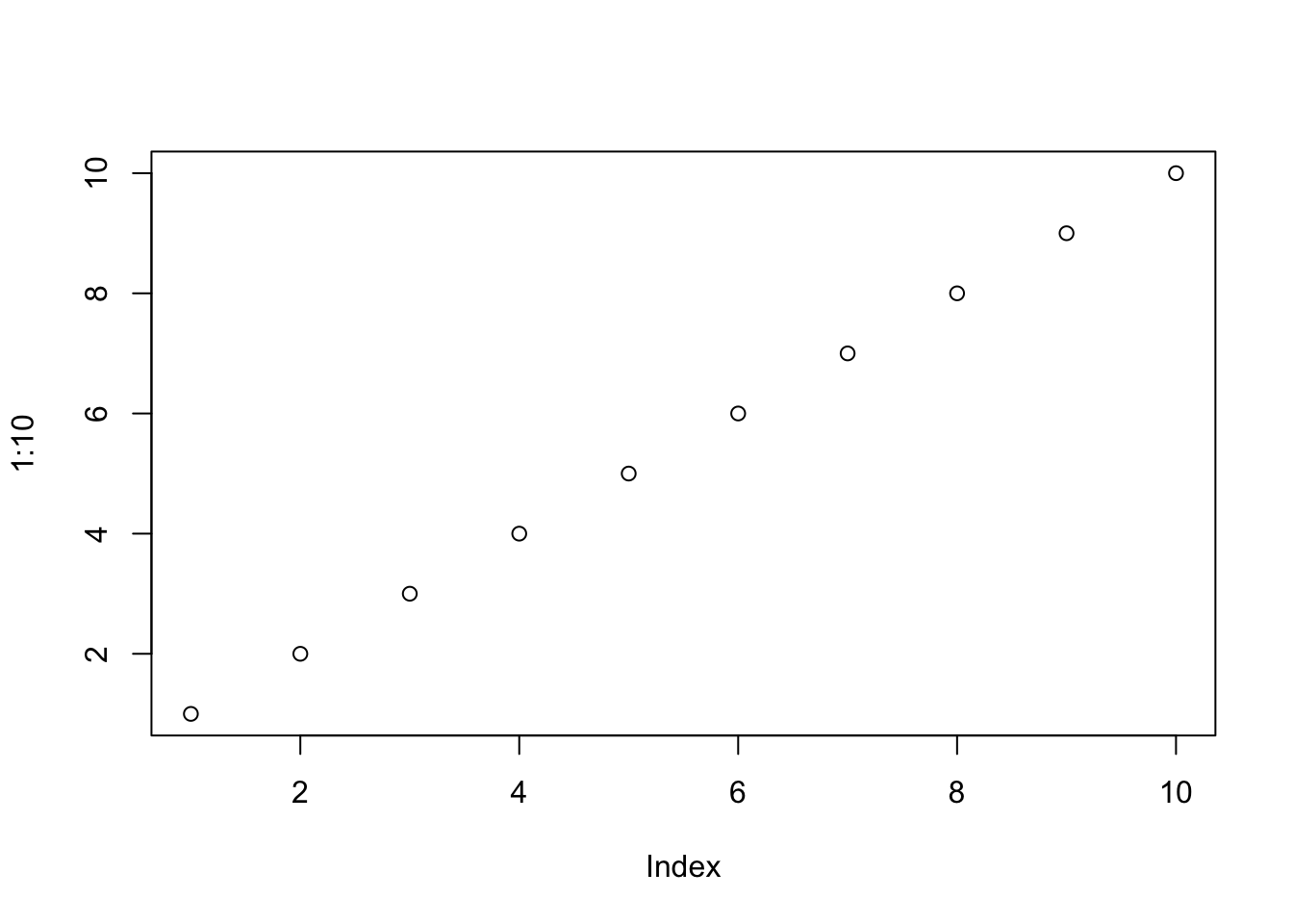
Figure 4: What a simple plot
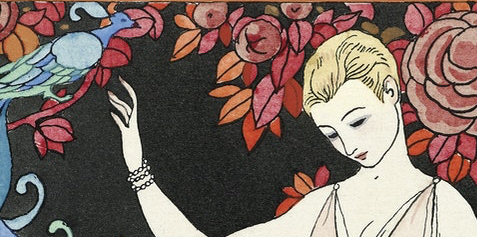
Side by side images
I couldn’t figure out how to use knitr::include_graphics using file paths, so one solution I found for using side by side plots was found
here which uses HTML code:
<img src="image1.png" width="425"/> <img src="image2.png" width="425"/>
For example:


knitr::include_graphics(c("/img/revoir.jpg","/img/arbre.jpg"), error = FALSE)
References
https://rmarkdown.rstudio.com/authoring_basics.html
- Posted on:
- July 9, 2021
- Length:
- 15 minute read, 3168 words
- Categories:
- Personal
- Tags:
- blogdown cheatsheet Rmarkdown